Introduction
US News reports that the United States has nearly 4000 degree-granting institutions as of 2020. In addition to degree-granting colleges and universities, there are hundreds of other post-secondary schools that provide students with certifications and professional licenses. With such a wide variety of post-secondary options, students have to pay close attention to the various distinctions that make these schools unique. Although the US Department of Education collects data on hundreds of institutional attributes, students only really consider a few of these variables. Some of the common considerations are ranking, size, diversity, student life, and program success.
One variable that stands out is whether or not a school is a single-sex institution. Given the history of mixed-sex education and the progression of women’s rights in the United States, single-sex education might seem like a relic of the past, but there are still a few dozen institutions that are committed to keeping genders separate.
With this in mind, this project will try to examine some of the key differences between co-ed and single-sex colleges. We will be using the US Department of Education’s college-scorecard data set, which contains all of the possible institution-level data one could ask for.
This is a very long analysis, so for a summary of all the findings, skip to the conclusion.
Data Preparation
Here, let’s unpack the data set by selecting relevant
variables.
setwd("C:/Users/laryl/Desktop/Data Sets/College Score Card")

library(data.table)
college_scorecard_raw <- fread("Most-Recent-Cohorts-All-Data-Elements.csv",
                                       select = c('INSTNM', 'MENONLY', 'WOMENONLY','CURROPER', # Institutional Attributes
                                                  'LATITUDE','LONGITUDE', # Geography

                                                  'HBCU','PBI', 'ANNHI', 'TRIBAL', 'AANAPII',
                                                  'HSI','NANTI','RELAFFIL', # Categorical Demographics

                                                  'UGDS', 'UGDS_WHITE', 'UGDS_BLACK', 'UGDS_HISP','UGDS_ASIAN',
                                                  'UGDS_AIAN','UGDS_NHPI','UGDS_2MOR','UGDS_NRA','UGDS_UNKN', # Numerical Demographics

                                                  'ADM_RATE', 'ADM_RATE_ALL',  'SATVRMID', 'SATMTMID',
                                                  'SATWRMID', 'ACTCMMID', 'ACTENMID',
                                                  'ACTMTMID', 'ACTWRMID', 'SAT_AVG', 'SAT_AVG_ALL', # Admission Statistics

                                                  'PCIP01', 'PCIP03', 'PCIP04', 'PCIP05', 'PCIP09', 'PCIP10', 'PCIP11', 'PCIP12',
                                                  'PCIP13', 'PCIP14', 'PCIP15', 'PCIP16', 'PCIP19', 'PCIP22',
                                                  'PCIP23', 'PCIP24', 'PCIP25', 'PCIP26', 'PCIP27',
                                                  'PCIP29', 'PCIP30', 'PCIP31', 'PCIP38', 'PCIP39',
                                                  'PCIP40', 'PCIP41', 'PCIP42', 'PCIP43','PCIP44', 'PCIP45', 'PCIP46', 'PCIP47', 'PCIP48',                                                      'PCIP49', 'PCIP50', 'PCIP51', 'PCIP52', 'PCIP54', # Percentage of Majors

                                                  'MN_EARN_WNE_P10', 'MD_EARN_WNE_P10', # Earnings After College

                                                  'AVGFACSAL', 'PFTFAC', # Faculty Employment

                                                  'C150_4','C150_4_WHITE', 'C150_4_BLACK', 'C150_4_HISP',
                                                  'C150_4_ASIAN', 'C150_4_AIAN', 'C150_4_NHPI',
                                                  'C150_4_2MOR', 'C150_4_NRA', 'C150_4_UNKN', # Completion

                                                  'RET_FT4_POOLED', #Retention
                                                  'MEDIAN_HH_INC', 'LN_MEDIAN_HH_INC'))# Household Income

str(college_scorecard_raw)
## Classes 'data.table' and 'data.frame': 6806 obs. of 90 variables:
## $ INSTNM : chr "Alabama A & M University" "University of Alabama at Birmingham" "Amridge University" "University of Alabama in Huntsville" ...
## $ MENONLY : chr "0" "0" "0" "0" ...
## $ WOMENONLY : chr "0" "0" "0" "0" ...
## $ CURROPER : int 1 1 1 1 1 1 1 1 1 1 ...
## $ LATITUDE : chr "34.783368" "33.505697" "32.362609" "34.724557" ...
## $ LONGITUDE : chr "-86.568502" "-86.799345" "-86.17401" "-86.640449" ...
## $ HBCU : chr "1" "0" "0" "0" ...
## $ PBI : chr "0" "0" "1" "0" ...
## $ ANNHI : chr "0" "0" "0" "0" ...
## $ TRIBAL : chr "0" "0" "0" "0" ...
## $ AANAPII : chr "0" "0" "0" "0" ...
## $ HSI : chr "0" "0" "0" "0" ...
## $ NANTI : chr "0" "0" "0" "0" ...
## $ RELAFFIL : chr "NULL" "NULL" "74" "NULL" ...
## $ UGDS : chr "4990" "13186" "351" "7458" ...
## $ UGDS_WHITE : chr "0.0186" "0.5717" "0.2393" "0.7167" ...
## $ UGDS_BLACK : chr "0.912" "0.2553" "0.7151" "0.0969" ...
## $ UGDS_HISP : chr "0.0088" "0.0334" "0.0171" "0.0528" ...
## $ UGDS_ASIAN : chr "0.0018" "0.0633" "0.0057" "0.0381" ...
## $ UGDS_AIAN : chr "0.0022" "0.0034" "0.0057" "0.0095" ...
## $ UGDS_NHPI : chr "0.0016" "0.0002" "0" "0.0008" ...
## $ UGDS_2MOR : chr "0.0118" "0.0457" "0" "0.0296" ...
## $ UGDS_NRA : chr "0.007" "0.0213" "0" "0.0223" ...
## $ UGDS_UNKN : chr "0.0361" "0.0058" "0.0171" "0.0333" ...
## $ ADM_RATE : chr "0.8986" "0.9211" "NULL" "0.8087" ...
## $ ADM_RATE_ALL : chr "0.8986" "0.9211" "NULL" "0.8087" ...
## $ SATVRMID : chr "475" "555" "NULL" "630" ...
## $ SATMTMID : chr "465" "555" "NULL" "565" ...
## $ SATWRMID : chr "414" "NULL" "NULL" "NULL" ...
## $ ACTCMMID : chr "18" "25" "NULL" "28" ...
## $ ACTENMID : chr "17" "27" "NULL" "30" ...
## $ ACTMTMID : chr "17" "23" "NULL" "27" ...
## $ ACTWRMID : chr "NULL" "NULL" "NULL" "NULL" ...
## $ SAT_AVG : chr "957" "1220" "NULL" "1314" ...
## $ SAT_AVG_ALL : chr "957" "1220" "NULL" "1314" ...
## $ PCIP01 : chr "0.0394" "0" "0" "0" ...
## $ PCIP03 : chr "0.0237" "0" "0" "0" ...
## $ PCIP04 : chr "0.0039" "0" "0" "0" ...
## $ PCIP05 : chr "0" "0.0016" "0" "0" ...
## $ PCIP09 : chr "0" "0.0375" "0" "0.0194" ...
## $ PCIP10 : chr "0.0394" "0" "0" "0" ...
## $ PCIP11 : chr "0.0592" "0.0139" "0" "0.059" ...
## $ PCIP12 : chr "0" "0" "0" "0" ...
## $ PCIP13 : chr "0.071" "0.0717" "0" "0.0283" ...
## $ PCIP14 : chr "0.1183" "0.0813" "0" "0.2892" ...
## $ PCIP15 : chr "0.0197" "0" "0" "0" ...
## $ PCIP16 : chr "0" "0.004" "0" "0.017" ...
## $ PCIP19 : chr "0.0394" "0" "0.1846" "0" ...
## $ PCIP22 : chr "0" "0" "0" "0" ...
## $ PCIP23 : chr "0.0158" "0.0207" "0" "0.0153" ...
## $ PCIP24 : chr "0.0473" "0.0351" "0.0308" "0" ...
## $ PCIP25 : chr "0" "0" "0" "0" ...
## $ PCIP26 : chr "0.0927" "0.0876" "0" "0.0436" ...
## $ PCIP27 : chr "0.0059" "0.0112" "0" "0.0153" ...
## $ PCIP29 : chr "0" "0" "0" "0" ...
## $ PCIP30 : chr "0" "0" "0" "0.0008" ...
## $ PCIP31 : chr "0.002" "0" "0" "0.021" ...
## $ PCIP38 : chr "0" "0.0064" "0" "0.0024" ...
## $ PCIP39 : chr "0" "0" "0.2154" "0" ...
## $ PCIP40 : chr "0.0355" "0.0235" "0" "0.0307" ...
## $ PCIP41 : chr "0" "0.0008" "0" "0" ...
## $ PCIP42 : chr "0.0631" "0.0602" "0" "0.0202" ...
## $ PCIP43 : chr "0.0572" "0.0267" "0.1077" "0" ...
## $ PCIP44 : chr "0.0493" "0.0263" "0" "0" ...
## $ PCIP45 : chr "0.0355" "0.0315" "0" "0.0242" ...
## $ PCIP46 : chr "0" "0" "0" "0" ...
## $ PCIP47 : chr "0" "0" "0" "0" ...
## $ PCIP48 : chr "0" "0" "0" "0" ...
## $ PCIP49 : chr "0" "0" "0" "0" ...
## $ PCIP50 : chr "0.0237" "0.0339" "0" "0.038" ...
## $ PCIP51 : chr "0" "0.2255" "0" "0.1543" ...
## $ PCIP52 : chr "0.1578" "0.1908" "0.4615" "0.2108" ...
## $ PCIP54 : chr "0" "0.01" "0" "0.0105" ...
## $ MN_EARN_WNE_P10 : chr "35500" "48400" "47600" "52000" ...
## $ MD_EARN_WNE_P10 : chr "31000" "41200" "39600" "46700" ...
## $ AVGFACSAL : chr "7101" "10717" "4292" "9442" ...
## $ PFTFAC : chr "0.7411" "0.7766" "1" "0.6544" ...
## $ C150_4 : chr "0.2685" "0.5829" "0.4" "0.5187" ...
## $ C150_4_WHITE : chr "0.25" "0.5769" "0.6667" "0.5417" ...
## $ C150_4_BLACK : chr "0.2681" "0.5255" "0" "0.3956" ...
## $ C150_4_HISP : chr "0.25" "0.62" "NULL" "0.5714" ...
## $ C150_4_ASIAN : chr "NULL" "0.789" "NULL" "0.619" ...
## $ C150_4_AIAN : chr "NULL" "0.5" "NULL" "0.4286" ...
## $ C150_4_NHPI : chr "0" "1" "NULL" "NULL" ...
## $ C150_4_2MOR : chr "0.25" "0.6" "NULL" "0.2222" ...
## $ C150_4_NRA : chr "NULL" "0.7647" "NULL" "0.5" ...
## $ C150_4_UNKN : chr "0.375" "0.5" "0" "0.5882" ...
## $ RET_FT4_POOLED : chr "0.5978" "0.8303" "0.2143" "0.8269" ...
## $ MEDIAN_HH_INC : chr "49720.22" "55735.22" "53683.7" "58688.62" ...
## $ LN_MEDIAN_HH_INC: chr "10.75" "10.8599996566772" "10.8400001525878" "10.9300003051757" ...
## - attr(*, ".internal.selfref")=<externalptr>Clearly, 90 variables is a lot to consider. But as we move through
this analysis, some of the variables will be eliminated or fused with
other variables. For now, our concern is improving the data type of
these attributes. For whatever reason, the fread function
unpacked many of the numeric variables in the data set as character
variables. So our first step will be to change the attributes to their
appropriate types.
college_scorecard_clean <- college_scorecard_raw[, c(5:6, 15:90) :=lapply(.SD, as.numeric), .SDcols= c(5:6, 15:90 )]

str(college_scorecard_clean)
## Classes 'data.table' and 'data.frame': 6806 obs. of 90 variables:
## $ INSTNM : chr "Alabama A & M University" "University of Alabama at Birmingham" "Amridge University" "University of Alabama in Huntsville" ...
## $ MENONLY : chr "0" "0" "0" "0" ...
## $ WOMENONLY : chr "0" "0" "0" "0" ...
## $ CURROPER : int 1 1 1 1 1 1 1 1 1 1 ...
## $ LATITUDE : num 34.8 33.5 32.4 34.7 32.4 ...
## $ LONGITUDE : num -86.6 -86.8 -86.2 -86.6 -86.3 ...
## $ HBCU : chr "1" "0" "0" "0" ...
## $ PBI : chr "0" "0" "1" "0" ...
## $ ANNHI : chr "0" "0" "0" "0" ...
## $ TRIBAL : chr "0" "0" "0" "0" ...
## $ AANAPII : chr "0" "0" "0" "0" ...
## $ HSI : chr "0" "0" "0" "0" ...
## $ NANTI : chr "0" "0" "0" "0" ...
## $ RELAFFIL : chr "NULL" "NULL" "74" "NULL" ...
## $ UGDS : num 4990 13186 351 7458 3903 ...
## $ UGDS_WHITE : num 0.0186 0.5717 0.2393 0.7167 0.0167 ...
## $ UGDS_BLACK : num 0.912 0.2553 0.7151 0.0969 0.9352 ...
## $ UGDS_HISP : num 0.0088 0.0334 0.0171 0.0528 0.0095 0.0499 0.0239 0.0311 0.0117 0.0342 ...
## $ UGDS_ASIAN : num 0.0018 0.0633 0.0057 0.0381 0.0041 0.0116 0.0041 0.0073 0.0221 0.0236 ...
## $ UGDS_AIAN : num 0.0022 0.0034 0.0057 0.0095 0.0013 0.0035 0.0041 0.0143 0.004 0.0038 ...
## $ UGDS_NHPI : num 0.0016 0.0002 0 0.0008 0.0005 0.001 0 0.0011 0.0007 0.0005 ...
## $ UGDS_2MOR : num 0.0118 0.0457 0 0.0296 0.0102 0.0338 0.0058 0.0212 0.0393 0.0225 ...
## $ UGDS_NRA : num 0.007 0.0213 0 0.0223 0.0102 0.0183 0.0017 0 0.0488 0.049 ...
## $ UGDS_UNKN : num 0.0361 0.0058 0.0171 0.0333 0.0123 0.0045 0.0017 0.0322 0.0084 0.0036 ...
## $ ADM_RATE : num 0.899 0.921 NA 0.809 0.977 ...
## $ ADM_RATE_ALL : num 0.899 0.921 NA 0.809 0.977 ...
## $ SATVRMID : num 475 555 NA 630 480 590 NA NA 540 615 ...
## $ SATMTMID : num 465 555 NA 565 465 580 NA NA 525 615 ...
## $ SATWRMID : num 414 NA NA NA NA 540 NA NA NA 570 ...
## $ ACTCMMID : num 18 25 NA 28 18 27 NA NA 21 28 ...
## $ ACTENMID : num 17 27 NA 30 17 29 NA NA 21 29 ...
## $ ACTMTMID : num 17 23 NA 27 17 25 NA NA 19 26 ...
## $ ACTWRMID : num NA NA NA NA NA 8 NA NA NA 8 ...
## $ SAT_AVG : num 957 1220 NA 1314 972 ...
## $ SAT_AVG_ALL : num 957 1220 NA 1314 972 ...
## $ PCIP01 : num 0.0394 0 0 0 0 0 0 0 0 0.0414 ...
## $ PCIP03 : num 0.0237 0 0 0 0 0.0053 0 0 0.0217 0.0202 ...
## $ PCIP04 : num 0.0039 0 0 0 0 0 0 0 0 0.0181 ...
## $ PCIP05 : num 0 0.0016 0 0 0 0.0027 0 0 0 0 ...
## $ PCIP09 : num 0 0.0375 0 0.0194 0.0892 0.0973 0 0 0.0339 0.0566 ...
## $ PCIP10 : num 0.0394 0 0 0 0 0 0 0 0 0 ...
## $ PCIP11 : num 0.0592 0.0139 0 0.059 0.0585 ...
## $ PCIP12 : num 0 0 0 0 0 0 0.0092 0 0 0 ...
## $ PCIP13 : num 0.071 0.0717 0 0.0283 0.1169 ...
## $ PCIP14 : num 0.1183 0.0813 0 0.2892 0 ...
## $ PCIP15 : num 0.0197 0 0 0 0 0 0.0552 0 0 0 ...
## $ PCIP16 : num 0 0.004 0 0.017 0 0.0058 0 0 0.0041 0.0062 ...
## $ PCIP19 : num 0.0394 0 0.1846 0 0 ...
## $ PCIP22 : num 0 0 0 0 0 0 0 0 0 0 ...
## $ PCIP23 : num 0.0158 0.0207 0 0.0153 0.0123 0.0093 0 0.0369 0.0136 0.0102 ...
## $ PCIP24 : num 0.0473 0.0351 0.0308 0 0 ...
## $ PCIP25 : num 0 0 0 0 0 0 0 0 0 0 ...
## $ PCIP26 : num 0.0927 0.0876 0 0.0436 0.0831 ...
## $ PCIP27 : num 0.0059 0.0112 0 0.0153 0.0169 0.0076 0 0.0224 0.0041 0.0058 ...
## $ PCIP29 : num 0 0 0 0 0 0 0 0 0 0 ...
## $ PCIP30 : num 0 0 0 0.0008 0.02 0.0148 0.0529 0.0171 0.0217 0.02 ...
## $ PCIP31 : num 0.002 0 0 0.021 0.0108 0 0 0.0092 0.0474 0 ...
## $ PCIP38 : num 0 0.0064 0 0.0024 0 0.0016 0 0.0066 0 0.0021 ...
## $ PCIP39 : num 0 0 0.215 0 0 ...
## $ PCIP40 : num 0.0355 0.0235 0 0.0307 0.0231 0.0114 0 0.0013 0.0176 0.0092 ...
## $ PCIP41 : num 0e+00 8e-04 0e+00 0e+00 0e+00 0e+00 0e+00 0e+00 0e+00 0e+00 ...
## $ PCIP42 : num 0.0631 0.0602 0 0.0202 0.06 0.0376 0 0.0211 0.0379 0.0279 ...
## $ PCIP43 : num 0.0572 0.0267 0.1077 0 0.0938 ...
## $ PCIP44 : num 0.0493 0.0263 0 0 0.0646 0.0092 0 0 0 0.016 ...
## $ PCIP45 : num 0.0355 0.0315 0 0.0242 0.0138 0.0364 0 0.0211 0.0407 0.0337 ...
## $ PCIP46 : num 0 0 0 0 0 0 0 0 0 0 ...
## $ PCIP47 : num 0 0 0 0 0 0 0.0322 0 0 0 ...
## $ PCIP48 : num 0 0 0 0 0 ...
## $ PCIP49 : num 0e+00 0e+00 0e+00 0e+00 0e+00 0e+00 0e+00 0e+00 0e+00 2e-04 ...
## $ PCIP50 : num 0.0237 0.0339 0 0.038 0.0585 0.0244 0 0.0303 0.0298 0.0296 ...
## $ PCIP51 : num 0 0.226 0 0.154 0.168 ...
## $ PCIP52 : num 0.158 0.191 0.462 0.211 0.106 ...
## $ PCIP54 : num 0 0.01 0 0.0105 0.0046 0.0124 0 0.0079 0.0068 0.0087 ...
## $ MN_EARN_WNE_P10 : num 35500 48400 47600 52000 30600 51600 32400 42400 38000 56300 ...
## $ MD_EARN_WNE_P10 : num 31000 41200 39600 46700 27700 44500 27700 38700 33300 48800 ...
## $ AVGFACSAL : num 7101 10717 4292 9442 7754 ...
## $ PFTFAC : num 0.741 0.777 1 0.654 0.583 ...
## $ C150_4 : num 0.269 0.583 0.4 0.519 0.3 ...
## $ C150_4_WHITE : num 0.25 0.577 0.667 0.542 0.4 ...
## $ C150_4_BLACK : num 0.268 0.525 0 0.396 0.295 ...
## $ C150_4_HISP : num 0.25 0.62 NA 0.571 0.316 ...
## $ C150_4_ASIAN : num NA 0.789 NA 0.619 1 ...
## $ C150_4_AIAN : num NA 0.5 NA 0.429 0 ...
## $ C150_4_NHPI : num 0 1 NA NA 0 0.75 NA NA 0 NA ...
## $ C150_4_2MOR : num 0.25 0.6 NA 0.222 0.3 ...
## $ C150_4_NRA : num NA 0.765 NA 0.5 0.588 ...
## $ C150_4_UNKN : num 0.375 0.5 0 0.588 0.214 ...
## $ RET_FT4_POOLED : num 0.598 0.83 0.214 0.827 0.59 ...
## $ MEDIAN_HH_INC : num 49720 55735 53684 58689 46065 ...
## $ LN_MEDIAN_HH_INC: num 10.8 10.9 10.8 10.9 10.7 ...
## - attr(*, ".internal.selfref")=<externalptr>Our current data set has two columns that tell us the sex-specific status of our institutions (“MENONLY” and “WOMENONLY). Let’s take a look at what values these variables contain:
table(college_scorecard_clean$MENONLY)##
## 0 1 NULL
## 6270 61 475table(college_scorecard_clean$WOMENONLY)##
## 0 1 NULL
## 6296 35 475Although this is great information and we can see which colleges are male-only and female-only, there are a few problems. First, there are null values that are not beneficial to us. The second problem is the fact that we don’t need the variables to be separate from each other. That separation is going to make creating graphs later slightly more challenging. Lastly, there is no easy way to view co-ed colleges, as both columns only tell us whether a college is for a specific sex or not. This means there isn’t a clear way to quickly distinguish co-ed colleges from the other sex-specific colleges when using one of the columns.
Thus, our next block will eliminate the null values, fuse the MENONLY and WOMENONLY columns, and create a new category called “CO-ED.” We will also make sure the colleges are operational.
# Load data manipulation packages
library(dplyr)
library(tidyr)

# Get rid of nulls in both columns
college_scorecard_null_less <- college_scorecard_clean[MENONLY %in% c(0,1)][WOMENONLY %in% c(0,1)]

#Rename values so that instead of 1 = sex-specific and 0 = the other options, we have it clearly tell us that it the sex or other options
college_scorecard_rewritten<- college_scorecard_null_less %>%
  mutate(MENONLY = if_else(MENONLY == 0, 'NA', 'MENONLY')) %>%
  mutate(WOMENONLY = if_else(WOMENONLY == 0, 'NA', 'WOMENONLY'))

# Fuse columns
college_scorecard_fused <-  unite(college_scorecard_rewritten, MENONLY, WOMENONLY, col = "SEX_SPECIFIC", sep = "_")


# Rewrite categories so that we have are three distinct categories
college_scorecard_prepped <- college_scorecard_fused %>%
  mutate(SEX_SPECIFIC = dplyr::recode(SEX_SPECIFIC,
                            'MENONLY_NA' = 'MEN ONLY',
                            'NA_NA' = 'CO-ED',
                            'NA_WOMENONLY'= 'WOMEN ONLY' ))


# Filter for colleges that are operational
college_scorecard_completely_prepped <- college_scorecard_prepped[CURROPER == "1"]

table(college_scorecard_completely_prepped[["SEX_SPECIFIC"]])
##
## CO-ED MEN ONLY WOMEN ONLY
## 5950 61 35As we can see, there are 3 distinct categories in a single variable. We can now begin to get some insights from the data.
At a Glance
Before going any further, we should get a good glance at what our data set visually looks like. This may reveal information that might not be as apparent when looking at raw statistics. I think this is the perfect opportunity to create a map that shows the location of the colleges filtered by sex-specificity.
#Create three data sets, one for each sex-specific category
Coed<- college_scorecard_prepped[SEX_SPECIFIC == "CO-ED"]
Men_only <- college_scorecard_prepped[SEX_SPECIFIC == "MEN ONLY"]
Women_only <- college_scorecard_prepped[SEX_SPECIFIC == "WOMEN ONLY"]
Let’s create the map:
#Load map packages
library(leaflet)
library(leaflet.extras)
library(htmltools)

#Create Map
map <- leaflet() %>%
  addProviderTiles("CartoDB") %>%
  addCircleMarkers(data = Men_only,
                   radius = 1,
                   color = "#1298d0",
                   label = ~htmlEscape(Men_only[["INSTNM"]]),
                   group = "MEN ONLY") %>%
    addCircleMarkers(data = Women_only,
                   radius = 1,
                   color = "#cc8834",
                   label = ~htmlEscape(Women_only[["INSTNM"]]),
                   group = "WOMEN ONLY") %>%
    addCircleMarkers(data = Coed,
                   radius = 1,
                   color = "#f1cb35",
                   label = ~htmlEscape(Coed[["INSTNM"]]),
                   group = "CO-ED") %>%
  addLayersControl(overlayGroups = c("MEN ONLY", "WOMEN ONLY", "CO-ED"))%>%
  setView(lat = 39.8282, lng = -98.5795, zoom = 4)


#Display Map
map
This interactive map displays quite a bit of information. First, we can see the difference in the number of colleges there are in each of the categories by changing the layers in the top right corner. Additionally, we can see that most of the colleges that are sex-specific are concentrated along the eastern side of the United States. Moreover, as you hover over the male-only colleges you can see that many of them are religiously affiliated.
Key Variables
Now, we can begin to analyze some of the variables that might distinguish the sex-specific categories.
The variables are:
- Demographics (Categorically and Numerically)
- Admission Statistics
- Percentage of Degrees Awarded in Academic Divisions
- Completion Rates by Ethnicities
- Retention Rates
- Faculty Employment Information
- Household Income
Demographics
Starting with one of the categorical demographic variables, there are 8 columns of interest:
- HBCU (Flag for Historically Black College or University)
- PBI (Flag for predominantly black institution)
- ANNHI (Flag for Alaska Native Hawaiian serving institution)
- TRIBAL (Flag for tribal college and university)
- AANAPII (Flag for Asian American, Native American, and Pacific Islander-serving institution)
- HSI (Flag for Hispanic-serving institution)
- NANTI (Flag for Native American non-tribal institution)
- RELAFFIL (Religious affiliation of the institution)
Let’s take a look it look at what values one of these columns has.
table(college_scorecard_completely_prepped$PBI)##
## 0 1 NULL
## 5949 94 3Like the sex-specific variables above, we have null values which don’t give us useful information. Moreover, because there are so many categories, we don’t want to create a chart for each one. Instead, we will be fusing the first 7 variables that are flagged for particular ethnicities, just like we did for the sex-specific categories.
Additionally, because the religious column has dozens of categories, creating a chart for all of them does not make sense. Instead, we are going to collapse all of the categories into religious and non-religious.
# Data Manipulations
library(forcats)


# Change values so that they are strings
college_scorecard_cat_demographics_rw <- college_scorecard_completely_prepped %>%
  mutate(HBCU = dplyr::recode(HBCU,
                             '0' = 'Not HBCU',
                             '1' = 'HBCU',
                             'NULL'= 'Not HBCU' )) %>%
  mutate(PBI = dplyr::recode(PBI,
                             '0' = 'Not PBI',
                             '1' = 'PBI',
                             'NULL'= 'Not PBI' )) %>%
  mutate(ANNHI = dplyr::recode(ANNHI,
                             '0' = 'Not ANNHI',
                             '1' = 'ANNHI',
                             'NULL'= 'Not ANNHI' )) %>%
  mutate(TRIBAL = dplyr::recode(TRIBAL,
                             '0' = 'Not TRIBAL',
                             '1' = 'TRIBAL',
                             'NULL'= 'Not TRIBAL' )) %>%
  mutate(AANAPII = dplyr::recode(AANAPII,
                             '0' = 'Not AANAPII',
                             '1' = 'AANAPII',
                             'NULL'= 'Not AANAPII' )) %>%
  mutate(HSI = dplyr::recode(HSI,
                             '0' = 'Not HSI',
                             '1' = 'HSI',
                             'NULL'= 'Not HSI' )) %>%
  mutate(NANTI = dplyr::recode(NANTI,
                             '0' = 'Not NANTI',
                             '1' = 'NANTI',
                             'NULL'= 'Not NANTI' )) %>%
# Collapse categories so that we have No Affiliation and  Religious Affiliation
  mutate(RELAFFIL = fct_other(RELAFFIL,
                              keep = "NULL"))%>%
  mutate(RELAFFIL = dplyr::recode(RELAFFIL,
                           "NULL" = "No Affiliation",
                           "Other" = "Religious Affiliation"))

# Fuse categories into one variable
college_scorecard_cat_demographics_fused <-  unite(college_scorecard_cat_demographics_rw, HBCU, PBI, ANNHI, TRIBAL, AANAPII,HSI, NANTI, col = "DEMOGRAPHICS", sep = "/")

table(college_scorecard_cat_demographics_fused$DEMOGRAPHICS)
##
## HBCU/Not PBI/Not ANNHI/Not TRIBAL/Not AANAPII/Not HSI/Not NANTI
## 99
## Not HBCU/Not PBI/ANNHI/Not TRIBAL/AANAPII/Not HSI/Not NANTI
## 17
## Not HBCU/Not PBI/ANNHI/Not TRIBAL/Not AANAPII/HSI/NANTI
## 1
## Not HBCU/Not PBI/ANNHI/Not TRIBAL/Not AANAPII/Not HSI/NANTI
## 9
## Not HBCU/Not PBI/ANNHI/Not TRIBAL/Not AANAPII/Not HSI/Not NANTI
## 2
## Not HBCU/Not PBI/ANNHI/TRIBAL/AANAPII/Not HSI/Not NANTI
## 1
## Not HBCU/Not PBI/ANNHI/TRIBAL/Not AANAPII/Not HSI/Not NANTI
## 5
## Not HBCU/Not PBI/Not ANNHI/Not TRIBAL/AANAPII/HSI/Not NANTI
## 80
## Not HBCU/Not PBI/Not ANNHI/Not TRIBAL/AANAPII/Not HSI/Not NANTI
## 60
## Not HBCU/Not PBI/Not ANNHI/Not TRIBAL/Not AANAPII/HSI/NANTI
## 1
## Not HBCU/Not PBI/Not ANNHI/Not TRIBAL/Not AANAPII/HSI/Not NANTI
## 367
## Not HBCU/Not PBI/Not ANNHI/Not TRIBAL/Not AANAPII/Not HSI/NANTI
## 17
## Not HBCU/Not PBI/Not ANNHI/Not TRIBAL/Not AANAPII/Not HSI/Not NANTI
## 5264
## Not HBCU/Not PBI/Not ANNHI/TRIBAL/Not AANAPII/Not HSI/Not NANTI
## 29
## Not HBCU/PBI/Not ANNHI/Not TRIBAL/AANAPII/HSI/Not NANTI
## 1
## Not HBCU/PBI/Not ANNHI/Not TRIBAL/AANAPII/Not HSI/Not NANTI
## 1
## Not HBCU/PBI/Not ANNHI/Not TRIBAL/Not AANAPII/HSI/Not NANTI
## 8
## Not HBCU/PBI/Not ANNHI/Not TRIBAL/Not AANAPII/Not HSI/Not NANTI
## 84As we can see from the various categories that were created, there are many schools that fit into multiple categories. Again, having many categories does not give us a clear picture. The solution to this problem is to collapse the categories that have multiple flags into a single one called “Multiple.”
#Clean up categories
college_scorecard_cat_demographics_complete <-  college_scorecard_cat_demographics_fused %>%
  mutate(DEMOGRAPHICS = dplyr::recode(DEMOGRAPHICS,
                            'HBCU/Not PBI/Not ANNHI/Not TRIBAL/Not AANAPII/Not HSI/Not NANTI' = 'HBCU',
                            'Not HBCU/Not PBI/ANNHI/Not TRIBAL/Not AANAPII/HSI/NANTI' = 'ANNHI/HSI/NANTI',
                            'Not HBCU/Not PBI/ANNHI/Not TRIBAL/Not AANAPII/Not HSI/Not NANTI' = 'ANNHI',
                            'Not HBCU/Not PBI/ANNHI/TRIBAL/Not AANAPII/Not HSI/Not NANTI' = 'ANNHI/TRIBAL',
                            'Not HBCU/Not PBI/Not ANNHI/Not TRIBAL/AANAPII/Not HSI/Not NANTI' = 'AANAPII',
                            'Not HBCU/Not PBI/Not ANNHI/Not TRIBAL/Not AANAPII/HSI/Not NANTI' = 'HSI',
                            'Not HBCU/Not PBI/Not ANNHI/Not TRIBAL/Not AANAPII/Not HSI/Not NANTI' = 'None',
                            'Not HBCU/PBI/Not ANNHI/Not TRIBAL/AANAPII/HSI/Not NANTI'= 'PBI/AANAPII/HSI',
                            'Not HBCU/PBI/Not ANNHI/Not TRIBAL/Not AANAPII/HSI/Not NANTI' = 'PBI/HSI',

                            'Not HBCU/Not PBI/ANNHI/Not TRIBAL/AANAPII/Not HSI/Not NANTI' = 'ANNHI/AANAPII',
                            'Not HBCU/Not PBI/ANNHI/Not TRIBAL/Not AANAPII/Not HSI/NANTI' = 'ANNHI/NANTI',
                            'Not HBCU/Not PBI/ANNHI/TRIBAL/AANAPII/Not HSI/Not NANTI' = 'ANNHI/TRIBAL/AANAPII',
                            'Not HBCU/Not PBI/Not ANNHI/Not TRIBAL/AANAPII/HSI/Not NANTI' = 'AANAPII/HSI',
                            'Not HBCU/Not PBI/Not ANNHI/Not TRIBAL/Not AANAPII/HSI/NANTI'= 'HSI/NANTI',
                            'Not HBCU/Not PBI/Not ANNHI/Not TRIBAL/Not AANAPII/Not HSI/NANTI' = 'NANTI',
                            'Not HBCU/Not PBI/Not ANNHI/TRIBAL/Not AANAPII/Not HSI/Not NANTI' = 'TRIBAL',
                            'Not HBCU/PBI/Not ANNHI/Not TRIBAL/AANAPII/Not HSI/Not NANTI' = 'PBI/AANAPII',
                            'Not HBCU/PBI/Not ANNHI/Not TRIBAL/Not AANAPII/Not HSI/Not NANTI' = 'PBI')) %>%
  # Collapse all multi-categories into a single one
  mutate(DEMOGRAPHICS = fct_collapse(DEMOGRAPHICS,
                                     "Multiple" = c( 'ANNHI/HSI/NANTI', 'ANNHI/TRIBAL', 'PBI/AANAPII/HSI',
                                                     'PBI/HSI', 'ANNHI/AANAPII', 'ANNHI/NANTI',
                                                     'ANNHI/TRIBAL/AANAPII', 'AANAPII/HSI',
                                                     'HSI/NANTI', 'PBI/AANAPII'
                                                  )))

table(college_scorecard_cat_demographics_complete$DEMOGRAPHICS)
##
## AANAPII Multiple ANNHI HBCU HSI NANTI None PBI
## 60 124 2 99 367 17 5264 84
## TRIBAL
## 29The 18 categories have been reduced to 10. We can now proceed to the next phase, which is to produce a plot that will test if there is a relationship between sex-specificity and demographics. One of the options we can use to plot a categorical variable against another categorical variable is a mosaic plot.
library(vcd)
tbl_status<- xtabs(~ DEMOGRAPHICS + SEX_SPECIFIC, college_scorecard_cat_demographics_complete)
ftable(tbl_status)
## SEX_SPECIFIC CO-ED MEN ONLY WOMEN ONLY
## DEMOGRAPHICS
## AANAPII 59 0 1
## Multiple 122 0 2
## ANNHI 2 0 0
## HBCU 96 1 2
## HSI 365 0 2
## NANTI 17 0 0
## None 5176 60 28
## PBI 84 0 0
## TRIBAL 29 0 0mosaic(tbl_status,
labeling_args = list(rot_labels = c(top = 90, left = 0),
gp_labels=gpar(fontsize= 9),
offset_varnames = c(top = 2, left = 2), offset_labels = c(left = 0.5, top =2)),
spacing = spacing_increase(start = unit(0.45, "lines"), rate = 1),
margins = c(top = 0.25, bottom = 0.5),
gp = shading_hcl,
legend = T)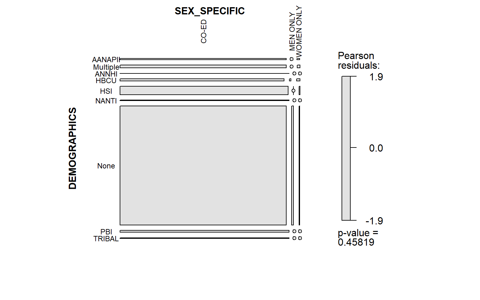 In this plot, each rectangle represents the intersection of 1 category
from one variable and another category from another variable. For
example, the largest rectangle represents the number of colleges that
are both co-ed and have no ethnic flag. The larger the area of the
rectangle, the more observations are in it. If there is no intersection
between the variable categories, a circle with a line is used.
In this plot, each rectangle represents the intersection of 1 category
from one variable and another category from another variable. For
example, the largest rectangle represents the number of colleges that
are both co-ed and have no ethnic flag. The larger the area of the
rectangle, the more observations are in it. If there is no intersection
between the variable categories, a circle with a line is used.
The Pearson residual colors, essentially, tell us whether we have more or fewer colleges than expected if we were to assume that demographics and sex-specificity are independent (as in there is no relationship). The presence of blue and red tells us that the variables are not independent meaning they have some kind of relationship. As we can clearly see in the plot, all of the rectangles are grey, which indicates that the two variables are independent.
Now, if we take a look at religious affiliation and plot it against sex-specificity, we might get something different.
tbl_status2<- xtabs(~ RELAFFIL +SEX_SPECIFIC, college_scorecard_cat_demographics_complete)
ftable(tbl_status2)
## SEX_SPECIFIC CO-ED MEN ONLY WOMEN ONLY
## RELAFFIL
## No Affiliation 5107 28 19
## Religious Affiliation 843 33 16mosaic(tbl_status2,
labeling_args = list(rot_labels = c(top = 90, left = 0),
gp_labels=gpar(fontsize= 8),
offset_varnames = c(top = 2, left = 4), offset_labels = c(left = 3, top =2)),
spacing = spacing_increase(start = unit(0.45, "lines"), rate = 1),
margins = c(top = 0.25, bottom = 0.5),
gp = shading_hcl,
legend = T)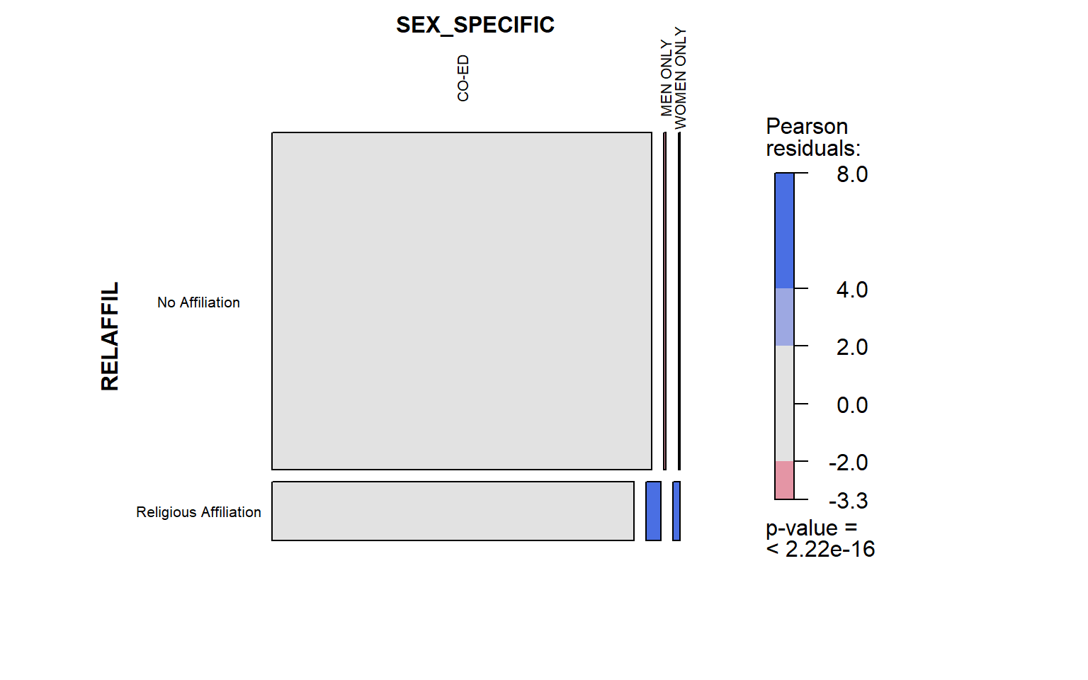 Now, we have some color! It looks like for men-only and women-only
colleges, there are more values than expected when they are religiously
affiliated. This matches some of the observations we made when we first
looked at the map.
Now, we have some color! It looks like for men-only and women-only
colleges, there are more values than expected when they are religiously
affiliated. This matches some of the observations we made when we first
looked at the map.
Let’s take a less confusing look by plotting the relationship between these two variables using an interactive stacked bar chart.
library(extrafont)
library(plotly)
plot_data <- college_scorecard_cat_demographics_complete %>%
  count(RELAFFIL, SEX_SPECIFIC) %>%
  add_count(SEX_SPECIFIC, wt= n) %>%
  mutate(percentage = (n/nn))


  plot_ly(x = plot_data[['SEX_SPECIFIC']], y = plot_data[['percentage']], color = plot_data[['RELAFFIL']], colors = c("#f1cb35",
"#cc8834")) %>%
  add_bars() %>%
  layout(barmode = "stack",
         font = list(family = "Georgia"),
         yaxis = list(title = "Percentage of Colleges", tickformat = "%"),
         xaxis = list(title= "College Type" ))
From this chart, we can clearly see that around half of both men-only and women-only colleges are religious wheres 14% percent of coed colleges are religious.
To continue our examination of the relationship between sex-specificity and demographics, we will be using a logistic regression framework. Specifically, we want to answer the question “does the proportion of ethnic groups help predict sex-specificity?”
From our data set there are a number of numeric demographic variables to examine:
- UGDS_WHITE (proportion of students that are white)
- UGDS_BLACK (proportion of students that are black)
- UGDS_HISP (proportion of students that are Hispanic )
- UGDS_ASIAN (proportion of students that are Asian )
- UGDS_AIAN (proportion of students that are American Indian/ Alaskan natives)
- UGDS_NHPI (proportion of students that Native Hawaiian/Pacific Islander)
- UGDS_2MOR (proportion of students that are 2 or more ethnicities)
- UGDS_NRA (proportion of students that are non-resident aliens [ I may refer to them as international])
- UGDS_UNKN (proportion of students with unknown race)
With so many variables to consider, the easiest way to investigate their relationship with sex-specificity is to create a logistic regression summary table and see which variables have the most significant relationships. Because we need the variables to be binary, we will be using one of the data sets from earlier on in our project. There are a few clean-up steps like making sure the MENONLY and WOMENONLY columns are numeric and have no null values.
#Make character variables to be numeric
college_scorecard_full_num_demographics<- college_scorecard_clean[, c(2:3) :=lapply(.SD, as.numeric), .SDcols= c(2:3)]

college_scorecard_dem_glance<- college_scorecard_full_num_demographics %>%
  select(UGDS, UGDS_WHITE, UGDS_BLACK, UGDS_HISP, UGDS_ASIAN,
          UGDS_AIAN, UGDS_NHPI, UGDS_2MOR, UGDS_NRA, UGDS_UNKN)

# Visualize Missing Values
library(visdat)
vis_miss(college_scorecard_dem_glance)+
  theme(axis.text.x = element_text(angle = 90, hjust = 0.65),
        text = element_text(family = "Georgia"))
Now our goal is to get rid of the missing rows so that we can run our logistic regression models.
college_scorecard_full_num_demographics2 <- college_scorecard_full_num_demographics %>%
  filter(UGDS != is.na(UGDS))


college_scorecard_dem_glance2<- college_scorecard_full_num_demographics2 %>%
  select(UGDS, UGDS_WHITE, UGDS_BLACK, UGDS_HISP, UGDS_ASIAN,
          UGDS_AIAN, UGDS_NHPI, UGDS_2MOR, UGDS_NRA, UGDS_UNKN)

vis_miss(college_scorecard_dem_glance2)+
  theme(axis.text.x = element_text(angle = 90, hjust = 0.65),
        text = element_text(family = "Georgia"))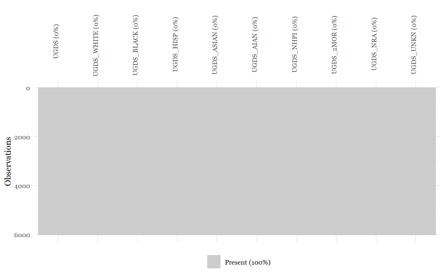
#Exclude non-operational colleges
college_scorecard_full_num_demographics_final<- college_scorecard_full_num_demographics2[CURROPER == "1"]
One important thing to address is the amount of colleges that were removed because of these clean up steps. We went from 6806 colleges to 5751. Because the missing values were consistent throughout these numeric demographics, the most likely reason they were left blank was because the researchers did not have access to the information.
First, we will create a table that shows the relationship between each explanatory numeric demographic variable and the MENONLY response variable.
library(broom)
#Create logistic regression model for predicting male-only colleges
demographics_mod_male1 <- tidy(glm(MENONLY ~  UGDS_WHITE,  family= binomial,  data = college_scorecard_full_num_demographics_final))

demographics_mod_male2 <- tidy(glm(MENONLY ~  UGDS_BLACK, family= binomial,  data = college_scorecard_full_num_demographics_final))


demographics_mod_male3 <- tidy(glm(MENONLY ~   UGDS_HISP, family= binomial,  data = college_scorecard_full_num_demographics_final))
demographics_mod_male4 <- tidy(glm(MENONLY ~   UGDS_ASIAN, family= binomial,  data = college_scorecard_full_num_demographics_final))

demographics_mod_male5 <- tidy(glm(MENONLY ~   UGDS_AIAN,  family= binomial,  data = college_scorecard_full_num_demographics_final))

demographics_mod_male6 <- tidy(glm(MENONLY ~  UGDS_NHPI,  family= binomial,  data = college_scorecard_full_num_demographics_final))

demographics_mod_male7 <- tidy(glm(MENONLY ~  UGDS_2MOR,  family= binomial,  data = college_scorecard_full_num_demographics_final))

demographics_mod_male8 <- tidy(glm(MENONLY ~  UGDS_NRA,  family= binomial,  data = college_scorecard_full_num_demographics_final))

demographics_mod_male9 <- tidy(glm(MENONLY ~  UGDS_UNKN,  family= binomial,  data = college_scorecard_full_num_demographics_final))

demographics_mod_male_main<-bind_rows(demographics_mod_male1, demographics_mod_male2, demographics_mod_male3,
          demographics_mod_male4, demographics_mod_male5, demographics_mod_male6,
          demographics_mod_male7, demographics_mod_male8, demographics_mod_male9)

demographics_mod_male_main
Because we cannot visualize a logistic regression that is more than 4 dimensions (3 explanatory variables and 1 response variable), we need to select the explanatory variables that are the most significant for our final model. There is also an extra incentive to get rid of some of these demographic variables because they are closely related and could create numerical instability. From this table, we can see that most of the explanatory variables independently have significant relationships with the MENONLY variable. The NRA variable and NHPI variables seem to have the least significant relationships with the MENONLY variable.
Now we will create a multivariate logistic model that takes into account all of the remaining variables to see if we can eliminate more explanatory variables.
demographics_mod_male_main2 <- glm(MENONLY ~   UGDS_WHITE +  UGDS_BLACK + UGDS_HISP + UGDS_ASIAN +
UGDS_AIAN +  UGDS_2MOR +  UGDS_UNKN, family= binomial,  data = college_scorecard_full_num_demographics_final)

summary(demographics_mod_male_main2)
##
## Call:
## glm(formula = MENONLY ~ UGDS_WHITE + UGDS_BLACK + UGDS_HISP +
## UGDS_ASIAN + UGDS_AIAN + UGDS_2MOR + UGDS_UNKN, family = binomial,
## data = college_scorecard_full_num_demographics_final)
##
## Deviance Residuals:
## Min 1Q Median 3Q Max
## -0.6941 -0.0479 -0.0128 -0.0023 5.4707
##
## Coefficients:
## Estimate Std. Error z value Pr(>|z|)
## (Intercept) -1.4389 0.8093 -1.778 0.075415 .
## UGDS_WHITE 0.1384 0.8362 0.166 0.868534
## UGDS_BLACK -10.8152 3.0340 -3.565 0.000364 ***
## UGDS_HISP -4.9057 1.5689 -3.127 0.001767 **
## UGDS_ASIAN -7.5415 5.6959 -1.324 0.185497
## UGDS_AIAN -201.6041 114.6773 -1.758 0.078746 .
## UGDS_2MOR -73.5400 20.1115 -3.657 0.000256 ***
## UGDS_UNKN -65.3860 28.0082 -2.335 0.019568 *
## ---
## Signif. codes: 0 '***' 0.001 '**' 0.01 '*' 0.05 '.' 0.1 ' ' 1
##
## (Dispersion parameter for binomial family taken to be 1)
##
## Null deviance: 648.63 on 5750 degrees of freedom
## Residual deviance: 364.70 on 5743 degrees of freedom
## AIC: 380.7
##
## Number of Fisher Scoring iterations: 13Here, some of these variables seem to have very large standard errors. The larger the standard error, the less precise the statistic, meaning the samples may not closely represent the population. A large standard error could be caused by having a small sample size, a large standard deviation, or a combination of both. To keep things simple, we will be removing the AIAN, 2MOR, and UNKN variables too because of their very large standard errors.
demographics_mod_male3 <- glm(MENONLY ~    UGDS_WHITE +  UGDS_BLACK + UGDS_HISP  +UGDS_ASIAN, family= binomial,  data = college_scorecard_full_num_demographics_final)

summary(demographics_mod_male3)
##
## Call:
## glm(formula = MENONLY ~ UGDS_WHITE + UGDS_BLACK + UGDS_HISP +
## UGDS_ASIAN, family = binomial, data = college_scorecard_full_num_demographics_final)
##
## Deviance Residuals:
## Min 1Q Median 3Q Max
## -0.5521 -0.1057 -0.0300 -0.0063 6.6810
##
## Coefficients:
## Estimate Std. Error z value Pr(>|z|)
## (Intercept) -6.932 2.089 -3.318 0.000907 ***
## UGDS_WHITE 5.128 2.153 2.382 0.017219 *
## UGDS_BLACK -16.316 5.175 -3.153 0.001618 **
## UGDS_HISP -2.536 3.505 -0.724 0.469364
## UGDS_ASIAN -21.548 12.738 -1.692 0.090718 .
## ---
## Signif. codes: 0 '***' 0.001 '**' 0.01 '*' 0.05 '.' 0.1 ' ' 1
##
## (Dispersion parameter for binomial family taken to be 1)
##
## Null deviance: 648.63 on 5750 degrees of freedom
## Residual deviance: 464.62 on 5746 degrees of freedom
## AIC: 474.62
##
## Number of Fisher Scoring iterations: 10Now, our table shows UGDS_ASIAN is not only statistically insignificant but also has a large standard error compared to the other three variables. Additionally, UGDS_HISP also appears to be statistically insignificant. With this in mind, our final model will only incorporate two variables (UGDS_WHITE and UGDS_BLACK).
But before we do the finalizing, we should perform a couple of steps. First, we should check if there is collinearity between our two variables so that it does not create instability in our model.
#Collinearity Check
college_scorecard_full_num_demographics_final %>%
  plot_ly(y = ~UGDS_BLACK, x= ~UGDS_WHITE, colors = "#44668b", text = ~INSTNM) %>%
  add_markers()
#Correlation Check
cor(college_scorecard_full_num_demographics_final$UGDS_WHITE, college_scorecard_full_num_demographics_final$UGDS_BLACK)## [1] -0.4719334So it looks like the variables are very correlated but not so much that they create instability.
Second, we should compare our model (with proportion of black and white students) to a model without black students so that we can see if the standard errors drastically change.
We are just going to rename the UGDS_BLACK variables so that our final plot is easier to to read.
# Rename variables
college_scorecard_full_num_demographics_final2 <- college_scorecard_full_num_demographics_final %>%
  rename( Black_Students = UGDS_BLACK)


#  Final Male Models
demographics_mod_male_final <- glm(MENONLY ~    UGDS_WHITE + Black_Students, family= binomial,
                                   data = college_scorecard_full_num_demographics_final2) # White and Black Students


demographics_mod_male_final2 <- glm(MENONLY ~    UGDS_WHITE,  family= binomial,
                                   data = college_scorecard_full_num_demographics_final2) # White Students Only
summary(demographics_mod_male_final)
##
## Call:
## glm(formula = MENONLY ~ UGDS_WHITE + Black_Students, family = binomial,
## data = college_scorecard_full_num_demographics_final2)
##
## Deviance Residuals:
## Min 1Q Median 3Q Max
## -0.5547 -0.1080 -0.0323 -0.0089 6.8577
##
## Coefficients:
## Estimate Std. Error z value Pr(>|z|)
## (Intercept) -9.667 1.343 -7.199 6.05e-13 ***
## UGDS_WHITE 7.873 1.434 5.492 3.98e-08 ***
## Black_Students -14.706 5.223 -2.816 0.00487 **
## ---
## Signif. codes: 0 '***' 0.001 '**' 0.01 '*' 0.05 '.' 0.1 ' ' 1
##
## (Dispersion parameter for binomial family taken to be 1)
##
## Null deviance: 648.63 on 5750 degrees of freedom
## Residual deviance: 468.47 on 5748 degrees of freedom
## AIC: 474.47
##
## Number of Fisher Scoring iterations: 10summary(demographics_mod_male_final2)##
## Call:
## glm(formula = MENONLY ~ UGDS_WHITE, family = binomial, data = college_scorecard_full_num_demographics_final2)
##
## Deviance Residuals:
## Min 1Q Median 3Q Max
## -0.5465 -0.1174 -0.0404 -0.0084 5.1060
##
## Coefficients:
## Estimate Std. Error z value Pr(>|z|)
## (Intercept) -13.072 1.108 -11.796 <2e-16 ***
## UGDS_WHITE 11.246 1.246 9.026 <2e-16 ***
## ---
## Signif. codes: 0 '***' 0.001 '**' 0.01 '*' 0.05 '.' 0.1 ' ' 1
##
## (Dispersion parameter for binomial family taken to be 1)
##
## Null deviance: 648.63 on 5750 degrees of freedom
## Residual deviance: 478.54 on 5749 degrees of freedom
## AIC: 482.54
##
## Number of Fisher Scoring iterations: 10The standard errors between models don’t differ much, so we are free to use our first one (with both black and white students).
Our final model shows that there is a significant relationship between being a men-only institution and particular proportions of certain ethnicities. Specifically, we can see that there is a positive relationship between men-only institutions and white students as well as a negative relationship between men-only institutions and black students. This finding does not seem too surprising because our map above showed that many of these institutions were seminary schools, which one can safely assume are mostly white men. But for the sake of transparency let’s take a quick look at a table of these institutions:
library(knitr)
Men_only_glance <- Men_only %>%
  select(INSTNM, UGDS_WHITE, UGDS_BLACK)

kable(Men_only_glance, col.names = c('Name', 'Prop. White', 'Prop. Black'), align = 'cc', caption = "Table 1.1 The Proportion of White and Black Students Per Institution")| Name | Prop. White | Prop. Black |
|---|---|---|
| Yeshiva Ohr Elchonon Chabad West Coast Talmudical Seminary | 0.9935 | 0.0000 |
| St. John Vianney College Seminary | 0.3333 | 0.0476 |
| Talmudic College of Florida | 0.8095 | 0.0000 |
| Morehouse College | 0.0032 | 0.9433 |
| Telshe Yeshiva-Chicago | 0.9870 | 0.0000 |
| Saint Meinrad School of Theology | NA | NA |
| Wabash College | 0.7446 | 0.0568 |
| Saint Joseph Seminary College | 0.6170 | 0.0071 |
| Ner Israel Rabbinical College | 0.9036 | 0.0000 |
| Pope St John XXIII National Seminary | NA | NA |
| Saint John’s Seminary | 0.5417 | 0.0000 |
| Saint Johns University | 0.7804 | 0.0456 |
| Conception Seminary College | 0.7000 | 0.0000 |
| Beth Medrash Govoha | 0.9683 | 0.0000 |
| Rabbinical College of America | 0.8438 | 0.0000 |
| Talmudical Academy-New Jersey | 0.9655 | 0.0000 |
| Beth Hamedrash Shaarei Yosher Institute | 1.0000 | 0.0000 |
| Central Yeshiva Tomchei Tmimim Lubavitz | 0.8374 | 0.0000 |
| Kehilath Yakov Rabbinical Seminary | 1.0000 | 0.0000 |
| Machzikei Hadath Rabbinical College | 0.9933 | 0.0000 |
| Mesivta Torah Vodaath Rabbinical Seminary | 1.0000 | 0.0000 |
| Mesivta of Eastern Parkway-Yeshiva Zichron Meilech | 1.0000 | 0.0000 |
| Mesivtha Tifereth Jerusalem of America | 0.9767 | 0.0000 |
| Mirrer Yeshiva Cent Institute | 0.9323 | 0.0000 |
| Ohr Hameir Theological Seminary | 0.9255 | 0.0000 |
| Rabbinical Academy Mesivta Rabbi Chaim Berlin | 0.9655 | 0.0000 |
| Rabbinical College Bobover Yeshiva Bnei Zion | 1.0000 | 0.0000 |
| Rabbinical College Beth Shraga | 1.0000 | 0.0000 |
| Rabbinical College of Long Island | 0.9872 | 0.0000 |
| Rabbinical Seminary of America | 1.0000 | 0.0000 |
| Sh’or Yoshuv Rabbinical College | 0.9493 | 0.0000 |
| Talmudical Seminary Oholei Torah | 0.9032 | 0.0000 |
| Talmudical Institute of Upstate New York | 1.0000 | 0.0000 |
| Torah Temimah Talmudical Seminary | 0.9524 | 0.0000 |
| United Talmudical Seminary | 0.9527 | 0.0000 |
| Yeshiva Karlin Stolin | 1.0000 | 0.0000 |
| Yeshiva Derech Chaim | 0.8182 | 0.0000 |
| Yeshiva of Nitra Rabbinical College | 0.9433 | 0.0000 |
| Yeshiva Shaar Hatorah | 1.0000 | 0.0000 |
| Yeshivath Viznitz | 1.0000 | 0.0000 |
| Yeshivath Zichron Moshe | 0.8933 | 0.0000 |
| Pontifical College Josephinum | 0.7444 | 0.0222 |
| Rabbinical College Telshe | 1.0000 | 0.0000 |
| Mount Angel Seminary | 0.2500 | 0.0000 |
| Saint Charles Borromeo Seminary-Overbrook | 0.6290 | 0.0968 |
| Talmudical Yeshiva of Philadelphia | 0.9593 | 0.0000 |
| Yeshivath Beth Moshe | 1.0000 | 0.0000 |
| Hampden-Sydney College | 0.8563 | 0.0485 |
| Sacred Heart Seminary and School of Theology | NA | NA |
| Bais Medrash Elyon | 1.0000 | 0.0000 |
| Yeshiva Gedolah of Greater Detroit | 1.0000 | 0.0000 |
| Yeshivah Gedolah Rabbinical College | 0.9118 | 0.0000 |
| Yeshiva Gedolah Imrei Yosef D’spinka | 1.0000 | 0.0000 |
| Yeshivas Novominsk | 0.9811 | 0.0000 |
| Rabbinical College of Ohr Shimon Yisroel | 1.0000 | 0.0000 |
| Yeshiva D’monsey Rabbinical College | 1.0000 | 0.0000 |
| Yeshiva of the Telshe Alumni | 1.0000 | 0.0000 |
| Yeshiva College of the Nations Capital | 1.0000 | 0.0000 |
| Yeshiva Shaarei Torah of Rockland | 0.9359 | 0.0000 |
| Beis Medrash Heichal Dovid | 1.0000 | 0.0000 |
| Uta Mesivta of Kiryas Joel | 0.9928 | 0.0000 |
For women-only colleges, we will follow a similar procedure.
#Create logistic regression model for predicting female-only colleges
demographics_mod_female1 <- tidy(glm(WOMENONLY ~  UGDS_WHITE,  family= binomial,  data = college_scorecard_full_num_demographics_final))

demographics_mod_female2 <- tidy(glm(WOMENONLY ~  UGDS_BLACK, family= binomial,  data = college_scorecard_full_num_demographics_final))


demographics_mod_female3 <- tidy(glm(WOMENONLY ~   UGDS_HISP, family= binomial,  data = college_scorecard_full_num_demographics_final))
demographics_mod_female4 <- tidy(glm(WOMENONLY ~   UGDS_ASIAN, family= binomial,  data = college_scorecard_full_num_demographics_final))

demographics_mod_female5 <- tidy(glm(WOMENONLY ~   UGDS_AIAN,  family= binomial,  data = college_scorecard_full_num_demographics_final))

demographics_mod_female6 <- tidy(glm(WOMENONLY ~  UGDS_NHPI,  family= binomial,  data = college_scorecard_full_num_demographics_final))

demographics_mod_female7 <- tidy(glm(WOMENONLY ~  UGDS_2MOR,  family= binomial,  data = college_scorecard_full_num_demographics_final))

demographics_mod_female8 <- tidy(glm(WOMENONLY ~  UGDS_NRA,  family= binomial,  data = college_scorecard_full_num_demographics_final))

demographics_mod_female9 <- tidy(glm(WOMENONLY ~  UGDS_UNKN,  family= binomial,  data = college_scorecard_full_num_demographics_final))

demographics_mod_female_main<-bind_rows(demographics_mod_female1, demographics_mod_female2, demographics_mod_female3,
          demographics_mod_female4, demographics_mod_female5, demographics_mod_female6,
          demographics_mod_female7, demographics_mod_female8, demographics_mod_female9)

demographics_mod_female_main
Based on some of the standard errors in this table, we will be getting rid of UGDS_AIAN and UGDS_NHPI. Additionally, there appears to be only two variables that are significant (UGDS_NRA, UGDS_2MOR).
demographics_mod_female_main <- glm(WOMENONLY ~  UGDS_2MOR + UGDS_NRA, family= binomial,  data = college_scorecard_full_num_demographics_final)

summary(demographics_mod_female_main)
##
## Call:
## glm(formula = WOMENONLY ~ UGDS_2MOR + UGDS_NRA, family = binomial,
## data = college_scorecard_full_num_demographics_final)
##
## Deviance Residuals:
## Min 1Q Median 3Q Max
## -0.5849 -0.1113 -0.1052 -0.0994 3.2663
##
## Coefficients:
## Estimate Std. Error z value Pr(>|z|)
## (Intercept) -5.3470 0.2078 -25.737 <2e-16 ***
## UGDS_2MOR 4.5186 2.4720 1.828 0.0676 .
## UGDS_NRA 2.8175 1.2308 2.289 0.0221 *
## ---
## Signif. codes: 0 '***' 0.001 '**' 0.01 '*' 0.05 '.' 0.1 ' ' 1
##
## (Dispersion parameter for binomial family taken to be 1)
##
## Null deviance: 426.91 on 5750 degrees of freedom
## Residual deviance: 421.33 on 5748 degrees of freedom
## AIC: 427.33
##
## Number of Fisher Scoring iterations: 8Because UGDS_2MOR did not reach our p-value threshold, we will exclude it from the final model.
demographics_mod_female_final <- glm(WOMENONLY ~ UGDS_NRA, family= binomial,  data = college_scorecard_full_num_demographics_final)

summary(demographics_mod_female_final)
##
## Call:
## glm(formula = WOMENONLY ~ UGDS_NRA, family = binomial, data = college_scorecard_full_num_demographics_final)
##
## Deviance Residuals:
## Min 1Q Median 3Q Max
## -0.4166 -0.1084 -0.1057 -0.1057 3.2217
##
## Coefficients:
## Estimate Std. Error z value Pr(>|z|)
## (Intercept) -5.1841 0.1791 -28.94 <2e-16 ***
## UGDS_NRA 2.7833 1.2046 2.31 0.0209 *
## ---
## Signif. codes: 0 '***' 0.001 '**' 0.01 '*' 0.05 '.' 0.1 ' ' 1
##
## (Dispersion parameter for binomial family taken to be 1)
##
## Null deviance: 426.91 on 5750 degrees of freedom
## Residual deviance: 423.62 on 5749 degrees of freedom
## AIC: 427.62
##
## Number of Fisher Scoring iterations: 8Based on this table, we can conclude that there is a significant relationship between proportion of nonresident alien students and women-only colleges. This finding was unexpected. I think a look at what is going on would be helpful:
library(knitr)
Women_only_glance <- Women_only %>%
  select(INSTNM, UGDS_NRA)


kable(Women_only_glance, col.names = c('Name', 'Prop. Nonresident Aliens'), align = 'cc', caption = "Table 1.2 The Proportion of Nonresident Students Per Institution")| Name | Prop. Nonresident Aliens |
|---|---|
| Judson College | 0.0000 |
| Mills College | 0.0119 |
| Mount Saint Mary’s University | 0.0009 |
| Scripps College | 0.0487 |
| Trinity Washington University | 0.0051 |
| Agnes Scott College | 0.0652 |
| Brenau University | 0.0498 |
| Spelman College | 0.0074 |
| Wesleyan College | 0.0916 |
| Saint Mary’s College | 0.0097 |
| Notre Dame of Maryland University | 0.0132 |
| Bay Path University | 0.0047 |
| Mount Holyoke College | 0.2717 |
| Simmons University | 0.0497 |
| Smith College | 0.1378 |
| Wellesley College | 0.1355 |
| College of Saint Benedict | 0.0438 |
| St Catherine University | 0.0065 |
| Cottey College | 0.1218 |
| Stephens College | 0.0018 |
| College of Saint Mary | 0.0111 |
| Barnard College | 0.0974 |
| Bennett College | 0.0000 |
| Meredith College | 0.0141 |
| Salem College | 0.0000 |
| Ursuline College | 0.0209 |
| Bryn Mawr College | 0.2151 |
| Cedar Crest College | 0.0890 |
| Moore College of Art and Design | 0.0161 |
| Converse College | 0.0571 |
| Hollins University | 0.0661 |
| Mary Baldwin University | 0.0072 |
| Sweet Briar College | 0.0256 |
| Alverno College | 0.0017 |
| Mount Mary University | 0.0132 |
nra_avges <- college_scorecard_completely_prepped %>%
  select(SEX_SPECIFIC, UGDS_NRA) %>%
  group_by(SEX_SPECIFIC) %>%
  summarize( UGDS_NRA_AVG= mean(UGDS_NRA, na.rm = TRUE))

kable(nra_avges, col.names = c('Institution Type', 'Mean Proportion Nonresident Aliens'), align = 'cc', caption = "Table 1.3 The Average Proportion of Nonresident Students Per Type of Institution")| Institution Type | Mean Proportion Nonresident Aliens |
|---|---|
| CO-ED | 0.0216359 |
| MEN ONLY | 0.0446603 |
| WOMEN ONLY | 0.0488971 |
Although an average of 4.9 % of the student body being international does not seem like much, when compared to the other types of schools, it looks like women colleges have more international students.
library(visreg)
visreg(demographics_mod_male_final, "UGDS_WHITE", by = "Black_Students",
       rug = FALSE ,
       band= FALSE,
       xlab = "Proportion of White Students",
       ylab = "Probabiltiy of Men-Only College",
       line= list(col ="#1298d0"),
       scale="response",
       gg = TRUE)+
  theme_bw()+
  labs(title = "Logistic Regression Prediction of Being Men-Only College")+
  theme(legend.position = "none",
        text = element_text(family = "Georgia"),
        plot.title = element_text(size = 15, margin(b = 10), hjust = 0.5, family = "Georgia"),
        strip.background = element_rect(
        color="Black", fill="#1298d0",  linetype="solid"))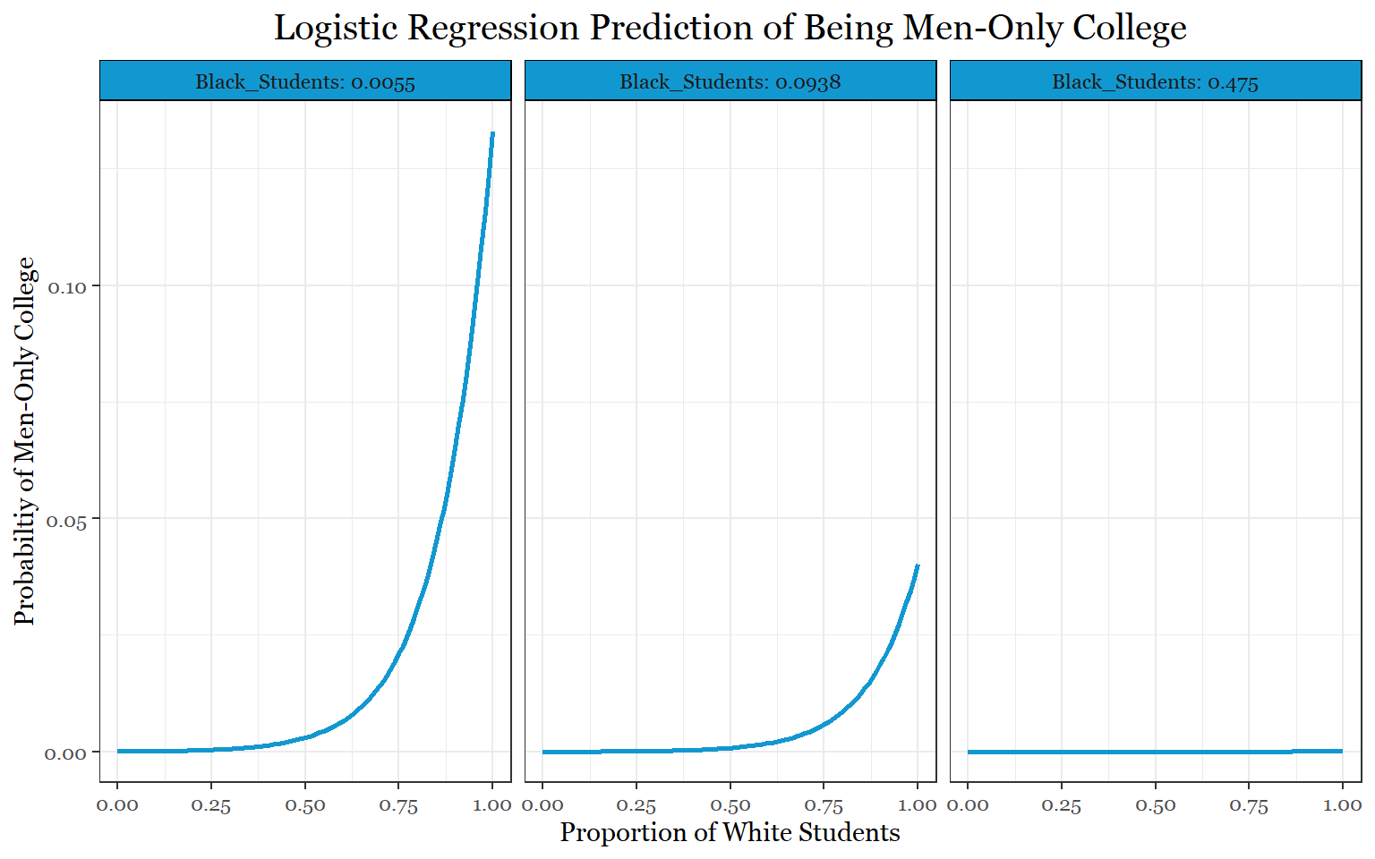
visreg(demographics_mod_female_final, "UGDS_NRA",
rug = FALSE ,
band= FALSE,
xlab = "Proportion of Nonresident Aliens",
ylab = "Probabiltiy of Being Women-Only College",
line= list(col ="#cc8834"),
scale="response",
gg = TRUE)+
theme_bw()+
labs(title = "Logistic Regression Prediction of Women-Only College")+
theme(legend.position = "none",
text = element_text(family = "Georgia"),
plot.title = element_text(size = 15, margin(b = 10), hjust = 0.5, family = "Georgia") )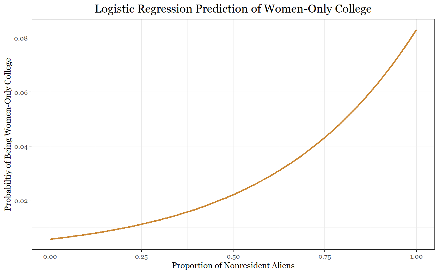 As we can see from the graphs, the relationships between these
demographic variables and sex-specificity are still fairly small despite
the statistical significance of the models. Testing the accuracy or
recall of the models does not seem appropriate given how weak the
relationships are.
As we can see from the graphs, the relationships between these
demographic variables and sex-specificity are still fairly small despite
the statistical significance of the models. Testing the accuracy or
recall of the models does not seem appropriate given how weak the
relationships are.
Admission Statistics
During the previous section, we had the numeric variable be the explanatory variable and the sex-specificity (a categorical variable) be the response variable. In this section and for the rest of the sections, sex-specificity is going to become the response variable. This transition was made, firstly, because creating logistic regression models for each one of these questions is going to be too much of a pain. Secondly, because these variables under investigation seem to have, for the most part, small relationships with gender, I feel the best thing would be to use a logistic regression framework using only the most significant variables. What would probably work best for an exploratory analysis like this one would be an anova framework that allows us to get a quick glance at the data using bar charts.
Our next step is to answer, “how do admission standards differ across the sex-specific colleges?”
Here are our explanatory variables:
- ADM_RATE (Admission Rate)
- SATVRMID (SAT Verbal Median)
- SATMTMID (SAT Math Median)
- SATWRMID (SAT Writing Median)
- SAT_AVG (SAT Overall Average)
- ACTCMMID (ACT Cumulative Median)
- ACTENMID (ACT English Median)
- ACTMTMID (ACT Math Median)
- ACTWRMID (ACT Writing Median)
Because there is a strong possibility that these variables will be collinear, it would be a good idea to take a look at what the overall averages are for each sex:
college_scorecard_completely_prepped %>%
  select(SEX_SPECIFIC,
         ADM_RATE,
         SATVRMID, SATMTMID, SAT_AVG,
         ACTCMMID, ACTENMID,
         ACTMTMID, ACTWRMID)%>%
  group_by(SEX_SPECIFIC)  %>%
  summarize(ADM_RATE = mean(ADM_RATE, na.rm= TRUE),
         SATVRMID= mean(SATVRMID, na.rm= TRUE),  SATMTMID= mean(SATMTMID, na.rm= TRUE), SAT_AVG= mean(SAT_AVG, na.rm= TRUE),
         ACTCMMID= mean(ACTCMMID, na.rm= TRUE), ACTENMID=  mean(ACTENMID, na.rm= TRUE),
         ACTMTMID= mean(ACTMTMID, na.rm= TRUE), ACTWRMID= mean(ACTWRMID, na.rm= TRUE)) %>%
kable(align = 'cc', caption = "Table 1.4 The Average Adission Statistics Per Type of Institution")| SEX_SPECIFIC | ADM_RATE | SATVRMID | SATMTMID | SAT_AVG | ACTCMMID | ACTENMID | ACTMTMID | ACTWRMID |
|---|---|---|---|---|---|---|---|---|
| CO-ED | 0.6768418 | 565.117 | 560.4017 | 1141.760 | 23.55411 | 23.28066 | 22.67185 | 7.688889 |
| MEN ONLY | 0.8322167 | 575.000 | 580.0000 | 1174.200 | 24.40000 | 23.60000 | 23.80000 | 7.666667 |
| WOMEN ONLY | 0.6096457 | 584.037 | 557.0370 | 1151.571 | 24.03571 | 24.48000 | 22.44000 | 8.600000 |
Women-only colleges being on average more selective is not surprising. With only 35 of them and there being very well known selective institutions like Scripps College and Barnard College, these findings were more or less expected. However, what came as a bit of a surprise was the selectivity of men-only colleges. Normally, as admission rates go down scores go up. Notice that the admission rates for men-only colleges is much higher than co-ed and women-only colleges. If men-only colleges are more selective, then we should see an admission rate under 60 percent. Additionally, since none of the men-only colleges are as selective as the most selective women-only colleges, what is driving these averages up so high?
Let’s take a look:
admissions_table <- function(sex) {
  college_scorecard_completely_prepped %>%
  filter(SEX_SPECIFIC == sex)  %>%
  select(INSTNM,
         ADM_RATE,
         SAT_AVG, SATVRMID, SATMTMID,
         ACTCMMID, ACTENMID,
         ACTMTMID, ACTWRMID) %>%
    kable(align = 'cc', caption = "Tables 1.4 Admission Statistics for Institution Type")
}

admissions_table("MEN ONLY")| INSTNM | ADM_RATE | SAT_AVG | SATVRMID | SATMTMID | ACTCMMID | ACTENMID | ACTMTMID | ACTWRMID |
|---|---|---|---|---|---|---|---|---|
| Yeshiva Ohr Elchonon Chabad West Coast Talmudical Seminary | 0.7113 | NA | NA | NA | NA | NA | NA | NA |
| St. John Vianney College Seminary | 1.0000 | NA | NA | NA | NA | NA | NA | NA |
| Talmudic College of Florida | NA | NA | NA | NA | NA | NA | NA | NA |
| Morehouse College | 0.5788 | 1120 | 560 | 550 | 23 | 23 | 22 | NA |
| Telshe Yeshiva-Chicago | 1.0000 | NA | NA | NA | NA | NA | NA | NA |
| Saint Meinrad School of Theology | NA | NA | NA | NA | NA | NA | NA | NA |
| Wabash College | 0.6497 | 1223 | 600 | 615 | 26 | 24 | 26 | 8 |
| Saint Joseph Seminary College | NA | NA | NA | NA | NA | NA | NA | NA |
| Ner Israel Rabbinical College | 0.8409 | NA | NA | NA | NA | NA | NA | NA |
| Pope St John XXIII National Seminary | NA | NA | NA | NA | NA | NA | NA | NA |
| Saint John’s Seminary | NA | NA | NA | NA | NA | NA | NA | NA |
| Saint Johns University | 0.7970 | 1209 | 560 | 585 | 25 | 24 | 25 | 8 |
| Conception Seminary College | 1.0000 | 1155 | NA | NA | 23 | 23 | 23 | 7 |
| Beth Medrash Govoha | NA | NA | NA | NA | NA | NA | NA | NA |
| Rabbinical College of America | 0.8732 | NA | NA | NA | NA | NA | NA | NA |
| Talmudical Academy-New Jersey | 0.8333 | NA | NA | NA | NA | NA | NA | NA |
| Beth Hamedrash Shaarei Yosher Institute | 0.7879 | NA | NA | NA | NA | NA | NA | NA |
| Central Yeshiva Tomchei Tmimim Lubavitz | 1.0000 | NA | NA | NA | NA | NA | NA | NA |
| Kehilath Yakov Rabbinical Seminary | NA | NA | NA | NA | NA | NA | NA | NA |
| Machzikei Hadath Rabbinical College | 0.9000 | NA | NA | NA | NA | NA | NA | NA |
| Mesivta Torah Vodaath Rabbinical Seminary | 0.6250 | NA | NA | NA | NA | NA | NA | NA |
| Mesivta of Eastern Parkway-Yeshiva Zichron Meilech | 0.8750 | NA | NA | NA | NA | NA | NA | NA |
| Mesivtha Tifereth Jerusalem of America | 0.9048 | NA | NA | NA | NA | NA | NA | NA |
| Mirrer Yeshiva Cent Institute | 0.7500 | NA | NA | NA | NA | NA | NA | NA |
| Ohr Hameir Theological Seminary | NA | NA | NA | NA | NA | NA | NA | NA |
| Rabbinical Academy Mesivta Rabbi Chaim Berlin | 1.0000 | NA | NA | NA | NA | NA | NA | NA |
| Rabbinical College Bobover Yeshiva Bnei Zion | NA | NA | NA | NA | NA | NA | NA | NA |
| Rabbinical College Beth Shraga | 1.0000 | NA | NA | NA | NA | NA | NA | NA |
| Rabbinical College of Long Island | 0.9778 | NA | NA | NA | NA | NA | NA | NA |
| Rabbinical Seminary of America | 0.9873 | NA | NA | NA | NA | NA | NA | NA |
| Sh’or Yoshuv Rabbinical College | 0.6667 | NA | NA | NA | NA | NA | NA | NA |
| Talmudical Seminary Oholei Torah | 0.9429 | NA | NA | NA | NA | NA | NA | NA |
| Talmudical Institute of Upstate New York | NA | NA | NA | NA | NA | NA | NA | NA |
| Torah Temimah Talmudical Seminary | 0.8000 | NA | NA | NA | NA | NA | NA | NA |
| United Talmudical Seminary | NA | NA | NA | NA | NA | NA | NA | NA |
| Yeshiva Karlin Stolin | 0.9574 | NA | NA | NA | NA | NA | NA | NA |
| Yeshiva Derech Chaim | 0.4861 | NA | NA | NA | NA | NA | NA | NA |
| Yeshiva of Nitra Rabbinical College | NA | NA | NA | NA | NA | NA | NA | NA |
| Yeshiva Shaar Hatorah | 0.8056 | NA | NA | NA | NA | NA | NA | NA |
| Yeshivath Viznitz | 0.9909 | NA | NA | NA | NA | NA | NA | NA |
| Yeshivath Zichron Moshe | 0.4800 | NA | NA | NA | NA | NA | NA | NA |
| Pontifical College Josephinum | 0.8333 | NA | NA | NA | NA | NA | NA | NA |
| Rabbinical College Telshe | 0.8400 | NA | NA | NA | NA | NA | NA | NA |
| Mount Angel Seminary | 1.0000 | NA | NA | NA | NA | NA | NA | NA |
| Saint Charles Borromeo Seminary-Overbrook | 0.9130 | NA | NA | NA | NA | NA | NA | NA |
| Talmudical Yeshiva of Philadelphia | 0.8444 | NA | NA | NA | NA | NA | NA | NA |
| Yeshivath Beth Moshe | 0.9091 | NA | NA | NA | NA | NA | NA | NA |
| Hampden-Sydney College | 0.5903 | 1164 | 580 | 570 | 25 | 24 | 23 | NA |
| Sacred Heart Seminary and School of Theology | NA | NA | NA | NA | NA | NA | NA | NA |
| Bais Medrash Elyon | 0.8000 | NA | NA | NA | NA | NA | NA | NA |
| Yeshiva Gedolah of Greater Detroit | 0.9375 | NA | NA | NA | NA | NA | NA | NA |
| Yeshivah Gedolah Rabbinical College | NA | NA | NA | NA | NA | NA | NA | NA |
| Yeshiva Gedolah Imrei Yosef D’spinka | NA | NA | NA | NA | NA | NA | NA | NA |
| Yeshivas Novominsk | 0.9833 | NA | NA | NA | NA | NA | NA | NA |
| Rabbinical College of Ohr Shimon Yisroel | NA | NA | NA | NA | NA | NA | NA | NA |
| Yeshiva D’monsey Rabbinical College | 0.5313 | NA | NA | NA | NA | NA | NA | NA |
| Yeshiva of the Telshe Alumni | 0.7857 | NA | NA | NA | NA | NA | NA | NA |
| Yeshiva College of the Nations Capital | NA | NA | NA | NA | NA | NA | NA | NA |
| Yeshiva Shaarei Torah of Rockland | NA | NA | NA | NA | NA | NA | NA | NA |
| Beis Medrash Heichal Dovid | 0.7636 | NA | NA | NA | NA | NA | NA | NA |
| Uta Mesivta of Kiryas Joel | NA | NA | NA | NA | NA | NA | NA | NA |
admissions_table("WOMEN ONLY")| INSTNM | ADM_RATE | SAT_AVG | SATVRMID | SATMTMID | ACTCMMID | ACTENMID | ACTMTMID | ACTWRMID |
|---|---|---|---|---|---|---|---|---|
| Judson College | 0.4820 | 1054 | 568 | 530 | 20 | 21 | 19 | NA |
| Mills College | 0.8554 | 1158 | 577 | 548 | 25 | 26 | 23 | NA |
| Mount Saint Mary’s University | 0.8382 | 1031 | 530 | 500 | 20 | NA | NA | NA |
| Scripps College | 0.2424 | 1409 | 700 | 690 | 32 | 34 | 29 | 9 |
| Trinity Washington University | 0.9512 | NA | NA | NA | NA | NA | NA | NA |
| Agnes Scott College | 0.7040 | NA | NA | NA | NA | NA | NA | NA |
| Brenau University | 0.5688 | 1031 | 525 | 495 | 20 | 20 | 19 | NA |
| Spelman College | 0.3934 | 1165 | 595 | 555 | 24 | 24 | 23 | NA |
| Wesleyan College | 0.4787 | 1030 | 535 | 485 | 20 | 20 | 18 | NA |
| Saint Mary’s College | 0.8190 | 1186 | 595 | 560 | 25 | 26 | 24 | NA |
| Notre Dame of Maryland University | 0.8763 | 1069 | 535 | 500 | 24 | NA | NA | NA |
| Bay Path University | 0.6041 | NA | NA | NA | NA | NA | NA | NA |
| Mount Holyoke College | 0.5091 | 1395 | 680 | 715 | 31 | 33 | 29 | NA |
| Simmons University | 0.6972 | 1228 | 620 | 595 | 27 | 28 | 25 | NA |
| Smith College | 0.3095 | NA | NA | NA | NA | NA | NA | NA |
| Wellesley College | 0.1954 | 1435 | 705 | 720 | 32 | 34 | 30 | 9 |
| College of Saint Benedict | 0.8338 | 1195 | 560 | 540 | 25 | 25 | 24 | 8 |
| St Catherine University | 0.7325 | 1124 | 619 | 572 | 22 | 21 | 21 | NA |
| Cottey College | 0.3804 | 1096 | 535 | 505 | 22 | 22 | 20 | NA |
| Stephens College | 0.5886 | 1138 | 575 | 515 | 23 | 23 | 20 | NA |
| College of Saint Mary | 0.5210 | NA | NA | NA | NA | NA | NA | NA |
| Barnard College | 0.1392 | 1422 | 705 | 710 | 32 | 34 | 30 | NA |
| Bennett College | 0.9634 | 911 | 465 | 435 | 17 | 16 | 17 | NA |
| Meredith College | 0.6257 | 1117 | 560 | 540 | 23 | 21 | 22 | NA |
| Salem College | 0.3947 | 1183 | 585 | 570 | 25 | 27 | 23 | NA |
| Ursuline College | 0.9034 | 1102 | 550 | 540 | 22 | 21 | 21 | 8 |
| Bryn Mawr College | 0.3408 | NA | NA | NA | NA | NA | NA | 9 |
| Cedar Crest College | 0.5719 | 1065 | 540 | 515 | 22 | 22 | 21 | NA |
| Moore College of Art and Design | 0.5195 | 1194 | 615 | 565 | 27 | NA | NA | NA |
| Converse College | 0.5852 | 1129 | 570 | 550 | 23 | 23 | 21 | NA |
| Hollins University | 0.6392 | 1204 | 610 | 565 | 27 | 28 | 22 | NA |
| Mary Baldwin University | 0.9991 | 1053 | 540 | 500 | 21 | 21 | 20 | NA |
| Sweet Briar College | 0.7569 | 1120 | 575 | 525 | 23 | 24 | 22 | NA |
| Alverno College | 0.6978 | NA | NA | NA | NA | NA | NA | NA |
| Mount Mary University | 0.6198 | 1000 | NA | NA | 19 | 18 | 18 | NA |
I knew it! Something was indeed going on here! Because most of the male colleges have NA’s, for their admission test statistics, only 5/61 contributed their numbers to those averages. This means that while most of the women-only college standards were averaged, only the more selective men-only college averages were used. This also makes sense because if most of your colleges are seminary schools, how could your average be so high?
This finding actually makes our job easier because the only valid variable to use is admission rate given the scarcity of data for the admission tests.
summary( lm( ADM_RATE ~ SEX_SPECIFIC, data= college_scorecard_completely_prepped ))##
## Call:
## lm(formula = ADM_RATE ~ SEX_SPECIFIC, data = college_scorecard_completely_prepped)
##
## Residuals:
## Min 1Q Median 3Q Max
## -0.67684 -0.12459 0.02196 0.16496 0.38945
##
## Coefficients:
## Estimate Std. Error t value Pr(>|t|)
## (Intercept) 0.676842 0.004976 136.027 < 2e-16 ***
## SEX_SPECIFICMEN ONLY 0.155375 0.033817 4.595 4.61e-06 ***
## SEX_SPECIFICWOMEN ONLY -0.067196 0.036978 -1.817 0.0693 .
## ---
## Signif. codes: 0 '***' 0.001 '**' 0.01 '*' 0.05 '.' 0.1 ' ' 1
##
## Residual standard error: 0.2168 on 1972 degrees of freedom
## (4071 observations deleted due to missingness)
## Multiple R-squared: 0.0124, Adjusted R-squared: 0.01139
## F-statistic: 12.38 on 2 and 1972 DF, p-value: 4.556e-06Here, we can clearly see that there is a significant positive relationship between admission rates and men-only institutions. Although women colleges did not cross the significance threshold, you can clearly see that there is a negative relationship between admission rate and women-only colleges.
Majors
For this section, I had two interesting questions:
Does attending a sex-specific school affect degree outcomes? Does going to a women-only college affect STEM degree outcomes?
Because the US Department of Education collects data on the percentage of students that graduate with particular majors, there are a lot of variables to work with!
However, since we are only interested in major academic divisions, we should be able to fuse most of these percentages and compare them that way. I decided to group them by three major divisions: Liberal Arts, STEM, and Professional/Vocational/Other.
Disclaimer: Many of these majors could have fit into a couple of groups, but in the interest of keeping things simple, I based my decisions mostly on this wikipedia page about academics fields.
Here is the breakdown of the variables:
STEM
- PCIP01 (agriculture)
- PCIP03 (Conservation)
- PCIP11 (computer science)
- PCIP14 (engineering)
- PCIP15 (engineering tech)
- PCIP26 (bio)
- PCIP27 (math)
- PCIP29 (applied science)
- PCIP40 (physics)
- PCIP41 (tech science)
- PCIP51 (health)
Professions, Vocations, and Other (everything I couldn t classify in the other 2)
- PCIP04 (architecture)
- PCIP09 (journalism/communication)
- PCIP10 (communications technology)
- PCIP12 (culinary)
- PCIP19 (consumer/human sciences)
- PCIP22 (legal)
- PCIP25 (library)
- PCIP30 (interdisciplinary)
- PCIP31 (recreation and fitness)
- PCIP43 (law enforcement/protective services)
- PCIP44 (social service)
- PCIP46 (construction)
- PCIP47 (mechanic)
- PCIP48 (precision production)
- PCIP49 (transportation/logistics)
- PCIP52 (business)
college_scorecard_majors<-  college_scorecard_completely_prepped %>%
  transmute(INSTNM,
            SEX_SPECIFIC ,
            LIB_ARTS = PCIP05 + PCIP13 + PCIP16 + PCIP23 + PCIP24 + PCIP38 + PCIP39 +PCIP42 + PCIP45 + PCIP50 + PCIP54,
            STEM = PCIP01 + PCIP03 + PCIP11 + PCIP14 + PCIP15 + PCIP26 + PCIP27+PCIP29 + PCIP40 +  PCIP41 +  PCIP51,
            PROF_VOC_OTHERS =  PCIP04 + PCIP09 + PCIP10 + PCIP12 + PCIP19 + PCIP22 +
              PCIP25 + PCIP30 + PCIP31 + PCIP43 + PCIP44 + PCIP46 + PCIP47 + PCIP48 + PCIP49 + PCIP52 )


kable(col.names = c("Name", 'Institution Type',  'Liberal Arts', 'STEM', "Professional & Vocation"), head(college_scorecard_majors),
align = 'cc', caption = "Table 1.5: Sample Proportion of Degree's Conferred Per Instituion")| Name | Institution Type | Liberal Arts | STEM | Professional & Vocation |
|---|---|---|---|---|
| Alabama A & M University | CO-ED | 0.2564 | 0.3944 | 0.3490 |
| University of Alabama at Birmingham | CO-ED | 0.2751 | 0.4438 | 0.2813 |
| Amridge University | CO-ED | 0.2462 | 0.0000 | 0.7538 |
| University of Alabama in Huntsville | CO-ED | 0.1559 | 0.5921 | 0.2520 |
| Alabama State University | CO-ED | 0.2661 | 0.3493 | 0.3846 |
| The University of Alabama | CO-ED | 0.1945 | 0.2968 | 0.5086 |
summary(lm(LIB_ARTS ~ SEX_SPECIFIC, data = college_scorecard_majors)) ##
## Call:
## lm(formula = LIB_ARTS ~ SEX_SPECIFIC, data = college_scorecard_majors)
##
## Residuals:
## Min 1Q Median 3Q Max
## -0.9298 -0.2005 -0.1551 0.1407 0.7996
##
## Coefficients:
## Estimate Std. Error t value Pr(>|t|)
## (Intercept) 0.200534 0.003495 57.374 < 2e-16 ***
## SEX_SPECIFICMEN ONLY 0.729223 0.034722 21.002 < 2e-16 ***
## SEX_SPECIFICWOMEN ONLY 0.263843 0.044608 5.915 3.52e-09 ***
## ---
## Signif. codes: 0 '***' 0.001 '**' 0.01 '*' 0.05 '.' 0.1 ' ' 1
##
## Residual standard error: 0.2631 on 5756 degrees of freedom
## (287 observations deleted due to missingness)
## Multiple R-squared: 0.0761, Adjusted R-squared: 0.07578
## F-statistic: 237.1 on 2 and 5756 DF, p-value: < 2.2e-16summary(lm(STEM ~ SEX_SPECIFIC, data = college_scorecard_majors)) ##
## Call:
## lm(formula = STEM ~ SEX_SPECIFIC, data = college_scorecard_majors)
##
## Residuals:
## Min 1Q Median 3Q Max
## -0.34488 -0.34488 -0.06808 0.17039 0.65512
##
## Coefficients:
## Estimate Std. Error t value Pr(>|t|)
## (Intercept) 0.344879 0.004443 77.621 < 2e-16 ***
## SEX_SPECIFICMEN ONLY -0.327114 0.044139 -7.411 1.44e-13 ***
## SEX_SPECIFICWOMEN ONLY -0.011948 0.056706 -0.211 0.833
## ---
## Signif. codes: 0 '***' 0.001 '**' 0.01 '*' 0.05 '.' 0.1 ' ' 1
##
## Residual standard error: 0.3344 on 5756 degrees of freedom
## (287 observations deleted due to missingness)
## Multiple R-squared: 0.009455, Adjusted R-squared: 0.009111
## F-statistic: 27.47 on 2 and 5756 DF, p-value: 1.335e-12summary(lm(PROF_VOC_OTHERS ~ SEX_SPECIFIC, data = college_scorecard_majors)) ##
## Call:
## lm(formula = PROF_VOC_OTHERS ~ SEX_SPECIFIC, data = college_scorecard_majors)
##
## Residuals:
## Min 1Q Median 3Q Max
## -0.4500 -0.2691 -0.0723 0.3030 0.5501
##
## Coefficients:
## Estimate Std. Error t value Pr(>|t|)
## (Intercept) 0.449999 0.004682 96.114 < 2e-16 ***
## SEX_SPECIFICMEN ONLY -0.432007 0.046512 -9.288 < 2e-16 ***
## SEX_SPECIFICWOMEN ONLY -0.247279 0.059754 -4.138 3.55e-05 ***
## ---
## Signif. codes: 0 '***' 0.001 '**' 0.01 '*' 0.05 '.' 0.1 ' ' 1
##
## Residual standard error: 0.3524 on 5756 degrees of freedom
## (287 observations deleted due to missingness)
## Multiple R-squared: 0.01755, Adjusted R-squared: 0.0172
## F-statistic: 51.4 on 2 and 5756 DF, p-value: < 2.2e-16The liberal arts model shows that both men-only and women-only institutions have a positive relationship with proportion of liberal arts degrees. This makes sense because many of these institutions (especially men-only) award religious and humanities degrees. For the STEM model, both men-only and women-only colleges have a negative relationship with percentage of STEM degrees. However, only the men-only relationship with STEM degrees is significant. Lastly, both men-only and women-only institutions have significant negative relationships with the percentage of professional and vocational degrees (men-only more significant).
Let’s take a look at what this looks like visually:
college_scorecard_majors %>%
  group_by(SEX_SPECIFIC) %>%
  summarize(mean_stem = mean(STEM, na.rm= TRUE), mean_lb_arts = mean(LIB_ARTS, na.rm= TRUE),mean_prof_voc = mean(PROF_VOC_OTHERS, na.rm= TRUE)) %>%
  plot_ly(x = ~SEX_SPECIFIC, y = ~mean_stem, type= 'bar', name= 'STEM Degrees', marker = list(color = "#44668b")) %>%
  add_trace(y = ~mean_lb_arts, name= 'Liberal Arts Degrees', marker = list(color = "#f1cb35"))%>%
  add_trace(y = ~mean_prof_voc, name= 'Professional and Vocational Degrees', marker = list(color = "#bdb8b8"))%>%
  layout(barmode = "group",
         xaxis = list(title = "College Type"),
         yaxis = list(title = "Proportion of Degrees Conferred"),
         font = list(family = "Georgia"))
I think it is pretty safe to say that if you are attending one of these male-only colleges, you are probably going to end up with a liberal arts degree.
One limitation of these methods is the fact that we could not get data that showed the degrees conferred by gender for co-ed institutions. Although co-ed institutions give more STEM degrees than women-only colleges, we need to keep in mind that this is the average for both genders. Because the number of men in STEM is usually higher than women in general, we could hypothesize that the average proportion of degrees conferred to women in co-ed colleges is lower than what is seen above.
Earning Outcomes
Here, we want to know if earning outcomes are affected by sex-specific schools.
‘MN_EARN_WNE_P10’ (Mean earnings of students working and not enrolled 10 years after entry) ‘MD_EARN_WNE_P10’ (Median earnings of students working and not enrolled 10 years after entry)
earning_outcomes_table <- bind_rows(
tidy(lm(MN_EARN_WNE_P10 ~ SEX_SPECIFIC, data= college_scorecard_completely_prepped)),
tidy(lm(MD_EARN_WNE_P10~ SEX_SPECIFIC, data= college_scorecard_completely_prepped))
)

earning_outcomes_table
From this table, it looks like both mean and median earning outcomes are positively associated with women-only colleges, albeit slightly. Both measurements are negatively associated with men-only colleges, but they are insignificant. One thing to note is that the median outcome for men-only colleges is almost significant.
college_scorecard_completely_prepped %>%
  group_by(SEX_SPECIFIC) %>%
  summarize(avg_mean = mean(MN_EARN_WNE_P10, na.rm= TRUE),
            avg_md = mean(MD_EARN_WNE_P10, na.rm= TRUE)) %>%
  plot_ly(x = ~SEX_SPECIFIC, y = ~avg_mean, type= 'bar', name= 'Mean Earning ', marker = list(color = "#44668b")) %>%
  add_trace(y = ~avg_md, name= 'Median Earnings', marker = list(color = "#f1cb35"))%>%
  layout(barmode = "group",
         xaxis = list(title = "College Type"),
         yaxis = list(title = "Average Earnings After 10 Years"),
         font = list(family = "Georgia"))
Completion
Next, does being at a sex-specific school affect completion rates for different ethnic groups?
Variables:
C150_4_WHITE (Completion rate for first-time, full-time students at four-year institutions (150% of expected time to completion) for white students)
C150_4_BLACK (Completion rate for first-time, full-time students at four-year institutions (150% of expected time to completion) for black students)
C150_4_HISP (Completion rate for first-time, full-time students at four-year institutions (150% of expected time to completion) for Hispanic students)
C150_4_ASIAN (Completion rate for first-time, full-time students at four-year institutions (150% of expected time to completion) for Asian students)
C150_4_AIAN (Completion rate for first-time, full-time students at four-year institutions (150% of expected time to completion) for American Indian/Alaska Native students)
C150_4_NHPI (Completion rate for first-time, full-time students at four-year institutions (150% of expected time to completion) for Native Hawaiian/Pacific Islander students)
C150_4_2MOR (Completion rate for first-time, full-time students at four-year institutions (150% of expected time to completion) for students of two-or-more-races)
C150_4_NRA (Completion rate for first-time, full-time students at four-year institutions (150% of expected time to completion) for non-resident alien students)
C150_4_UNKN (Completion rate for first-time, full-time students at four-year institutions (150% of expected time to completion) for students whose race is unknown)
summary(lm(C150_4_WHITE~ SEX_SPECIFIC, data= college_scorecard_completely_prepped))##
## Call:
## lm(formula = C150_4_WHITE ~ SEX_SPECIFIC, data = college_scorecard_completely_prepped)
##
## Residuals:
## Min 1Q Median 3Q Max
## -0.64224 -0.14239 0.01976 0.15054 0.61240
##
## Coefficients:
## Estimate Std. Error t value Pr(>|t|)
## (Intercept) 0.542386 0.004963 109.294 < 2e-16 ***
## SEX_SPECIFICMEN ONLY -0.154786 0.031111 -4.975 7.04e-07 ***
## SEX_SPECIFICWOMEN ONLY 0.099857 0.039238 2.545 0.011 *
## ---
## Signif. codes: 0 '***' 0.001 '**' 0.01 '*' 0.05 '.' 0.1 ' ' 1
##
## Residual standard error: 0.2236 on 2113 degrees of freedom
## (3930 observations deleted due to missingness)
## Multiple R-squared: 0.01481, Adjusted R-squared: 0.01387
## F-statistic: 15.88 on 2 and 2113 DF, p-value: 1.433e-07summary(lm(C150_4_BLACK~ SEX_SPECIFIC, data= college_scorecard_completely_prepped))##
## Call:
## lm(formula = C150_4_BLACK ~ SEX_SPECIFIC, data = college_scorecard_completely_prepped)
##
## Residuals:
## Min 1Q Median 3Q Max
## -0.52134 -0.18285 -0.02405 0.16015 0.59495
##
## Coefficients:
## Estimate Std. Error t value Pr(>|t|)
## (Intercept) 0.405052 0.005715 70.875 < 2e-16 ***
## SEX_SPECIFICMEN ONLY 0.184268 0.112312 1.641 0.10102
## SEX_SPECIFICWOMEN ONLY 0.116285 0.042778 2.718 0.00662 **
## ---
## Signif. codes: 0 '***' 0.001 '**' 0.01 '*' 0.05 '.' 0.1 ' ' 1
##
## Residual standard error: 0.2508 on 1963 degrees of freedom
## (4080 observations deleted due to missingness)
## Multiple R-squared: 0.005079, Adjusted R-squared: 0.004065
## F-statistic: 5.01 on 2 and 1963 DF, p-value: 0.006753summary(lm(C150_4_HISP~ SEX_SPECIFIC, data= college_scorecard_completely_prepped))##
## Call:
## lm(formula = C150_4_HISP ~ SEX_SPECIFIC, data = college_scorecard_completely_prepped)
##
## Residuals:
## Min 1Q Median 3Q Max
## -0.58758 -0.16029 -0.00389 0.16911 0.52788
##
## Coefficients:
## Estimate Std. Error t value Pr(>|t|)
## (Intercept) 0.476089 0.005599 85.024 < 2e-16 ***
## SEX_SPECIFICMEN ONLY -0.003972 0.071672 -0.055 0.95581
## SEX_SPECIFICWOMEN ONLY 0.111494 0.042211 2.641 0.00832 **
## ---
## Signif. codes: 0 '***' 0.001 '**' 0.01 '*' 0.05 '.' 0.1 ' ' 1
##
## Residual standard error: 0.2475 on 1998 degrees of freedom
## (4045 observations deleted due to missingness)
## Multiple R-squared: 0.003483, Adjusted R-squared: 0.002486
## F-statistic: 3.492 on 2 and 1998 DF, p-value: 0.03063summary(lm(C150_4_ASIAN~ SEX_SPECIFIC, data= college_scorecard_completely_prepped))##
## Call:
## lm(formula = C150_4_ASIAN ~ SEX_SPECIFIC, data = college_scorecard_completely_prepped)
##
## Residuals:
## Min 1Q Median 3Q Max
## -0.65546 -0.17798 0.03312 0.23202 0.52488
##
## Coefficients:
## Estimate Std. Error t value Pr(>|t|)
## (Intercept) 0.566881 0.007266 78.020 <2e-16 ***
## SEX_SPECIFICMEN ONLY -0.091765 0.122158 -0.751 0.453
## SEX_SPECIFICWOMEN ONLY 0.088580 0.054137 1.636 0.102
## ---
## Signif. codes: 0 '***' 0.001 '**' 0.01 '*' 0.05 '.' 0.1 ' ' 1
##
## Residual standard error: 0.2987 on 1724 degrees of freedom
## (4319 observations deleted due to missingness)
## Multiple R-squared: 0.001888, Adjusted R-squared: 0.0007303
## F-statistic: 1.631 on 2 and 1724 DF, p-value: 0.1961summary(lm(C150_4_AIAN~ SEX_SPECIFIC, data= college_scorecard_completely_prepped))##
## Call:
## lm(formula = C150_4_AIAN ~ SEX_SPECIFIC, data = college_scorecard_completely_prepped)
##
## Residuals:
## Min 1Q Median 3Q Max
## -0.43186 -0.43186 -0.04886 0.31814 0.64444
##
## Coefficients:
## Estimate Std. Error t value Pr(>|t|)
## (Intercept) 0.43186 0.01007 42.887 <2e-16 ***
## SEX_SPECIFICMEN ONLY 0.17529 0.26375 0.665 0.506
## SEX_SPECIFICWOMEN ONLY -0.07630 0.09676 -0.789 0.430
## ---
## Signif. codes: 0 '***' 0.001 '**' 0.01 '*' 0.05 '.' 0.1 ' ' 1
##
## Residual standard error: 0.3727 on 1384 degrees of freedom
## (4659 observations deleted due to missingness)
## Multiple R-squared: 0.0007709, Adjusted R-squared: -0.0006731
## F-statistic: 0.5339 on 2 and 1384 DF, p-value: 0.5865Here is the summary of the summary tables:
White Student Completion Rate:
- significant negative relationship for men-only
- slightly significant positive relationship for women-only
Black Student Completion Rate:
- moderately significant positive relationship for women-only
Hispanic Student Completion Rate:
- moderately significant positive relationship for women-only
Asian Student Completion Rate:
- no significant relationship for both men-only and women-only colleges
American Indian/ Alaskan Native Student Completion Rate:
- no significant relationship for both men-only and women-only colleges
Here is what it looks like visually:
college_scorecard_completely_prepped %>%
  group_by(SEX_SPECIFIC) %>%
  summarize(avg_completion_w = mean(C150_4_WHITE, na.rm= TRUE),
            avg_completion_b = mean(C150_4_BLACK, na.rm= TRUE),
            avg_completion_h = mean(C150_4_HISP, na.rm= TRUE),
            avg_completion_as = mean(C150_4_ASIAN, na.rm= TRUE),
            avg_completion_ai = mean(C150_4_AIAN, na.rm= TRUE)) %>%
  plot_ly(x = ~SEX_SPECIFIC, y = ~avg_completion_w, type= 'bar', name= 'White', marker = list(color = "#44668b")) %>%
  add_trace(y = ~avg_completion_b, name= 'Black', marker = list(color = "#f1cb35"))%>%
  add_trace(y = ~avg_completion_h, name= 'Hispanic', marker = list(color = "#1298d0"))%>%
  add_trace(y = ~avg_completion_as, name= 'Asian', marker = list(color = "#cc8834"))%>%
  add_trace(y = ~avg_completion_ai, name= 'American Indian/ Alaska Native', marker = list(color = "#bdb8b8"))%>%
  layout(barmode = "group",
         xaxis = list(title = "College Type"),
         yaxis = list(title = "Average Completion Rate"),
font = list(family = "Georgia"))summary(lm(C150_4_NHPI~ SEX_SPECIFIC, data= college_scorecard_completely_prepped))##
## Call:
## lm(formula = C150_4_NHPI ~ SEX_SPECIFIC, data = college_scorecard_completely_prepped)
##
## Residuals:
## Min 1Q Median 3Q Max
## -0.61904 -0.44404 -0.04404 0.55596 0.55596
##
## Coefficients:
## Estimate Std. Error t value Pr(>|t|)
## (Intercept) 0.44404 0.01384 32.076 <2e-16 ***
## SEX_SPECIFICWOMEN ONLY 0.17501 0.15521 1.128 0.26
## ---
## Signif. codes: 0 '***' 0.001 '**' 0.01 '*' 0.05 '.' 0.1 ' ' 1
##
## Residual standard error: 0.409 on 878 degrees of freedom
## (5166 observations deleted due to missingness)
## Multiple R-squared: 0.001446, Adjusted R-squared: 0.0003085
## F-statistic: 1.271 on 1 and 878 DF, p-value: 0.2598summary(lm(C150_4_2MOR~ SEX_SPECIFIC, data= college_scorecard_completely_prepped))##
## Call:
## lm(formula = C150_4_2MOR ~ SEX_SPECIFIC, data = college_scorecard_completely_prepped)
##
## Residuals:
## Min 1Q Median 3Q Max
## -0.55539 -0.20622 0.02708 0.19378 0.52708
##
## Coefficients:
## Estimate Std. Error t value Pr(>|t|)
## (Intercept) 0.472925 0.006913 68.414 <2e-16 ***
## SEX_SPECIFICMEN ONLY 0.227075 0.198793 1.142 0.2535
## SEX_SPECIFICWOMEN ONLY 0.082466 0.049396 1.669 0.0952 .
## ---
## Signif. codes: 0 '***' 0.001 '**' 0.01 '*' 0.05 '.' 0.1 ' ' 1
##
## Residual standard error: 0.281 on 1684 degrees of freedom
## (4359 observations deleted due to missingness)
## Multiple R-squared: 0.002413, Adjusted R-squared: 0.001228
## F-statistic: 2.037 on 2 and 1684 DF, p-value: 0.1308summary(lm(C150_4_NRA~ SEX_SPECIFIC, data= college_scorecard_completely_prepped))##
## Call:
## lm(formula = C150_4_NRA ~ SEX_SPECIFIC, data = college_scorecard_completely_prepped)
##
## Residuals:
## Min 1Q Median 3Q Max
## -0.64515 -0.17095 0.03585 0.21235 0.71789
##
## Coefficients:
## Estimate Std. Error t value Pr(>|t|)
## (Intercept) 0.587646 0.007393 79.491 < 2e-16 ***
## SEX_SPECIFICMEN ONLY -0.305537 0.062997 -4.850 1.36e-06 ***
## SEX_SPECIFICWOMEN ONLY 0.057507 0.054682 1.052 0.293
## ---
## Signif. codes: 0 '***' 0.001 '**' 0.01 '*' 0.05 '.' 0.1 ' ' 1
##
## Residual standard error: 0.2867 on 1550 degrees of freedom
## (4493 observations deleted due to missingness)
## Multiple R-squared: 0.01575, Adjusted R-squared: 0.01448
## F-statistic: 12.4 on 2 and 1550 DF, p-value: 4.551e-06summary(lm(C150_4_UNKN~ SEX_SPECIFIC, data= college_scorecard_completely_prepped))##
## Call:
## lm(formula = C150_4_UNKN ~ SEX_SPECIFIC, data = college_scorecard_completely_prepped)
##
## Residuals:
## Min 1Q Median 3Q Max
## -0.59045 -0.22123 0.00957 0.21547 0.50957
##
## Coefficients:
## Estimate Std. Error t value Pr(>|t|)
## (Intercept) 0.490429 0.007379 66.459 <2e-16 ***
## SEX_SPECIFICMEN ONLY -0.144262 0.171801 -0.840 0.4012
## SEX_SPECIFICWOMEN ONLY 0.100025 0.058769 1.702 0.0889 .
## ---
## Signif. codes: 0 '***' 0.001 '**' 0.01 '*' 0.05 '.' 0.1 ' ' 1
##
## Residual standard error: 0.2973 on 1649 degrees of freedom
## (4394 observations deleted due to missingness)
## Multiple R-squared: 0.002189, Adjusted R-squared: 0.0009787
## F-statistic: 1.809 on 2 and 1649 DF, p-value: 0.1642Another summary of the summaries:
Native Hawaiian/Pacific Islander Completion Rate:
- no significant relationship for both men-only and women-only colleges
2 or More Races Completion Rate:
- no significant relationship for both men-only and women-only colleges
Nonresident Aliens Completion Rate:
- very significant negative relationship for men-only
Unknown Completion Rate:
- no significant relationship for both men-only and women-only colleges
Here is the visual:
college_scorecard_completely_prepped %>%
  group_by(SEX_SPECIFIC) %>%
  summarize(avg_completion_nhpi = mean(C150_4_NHPI, na.rm= TRUE),
            avg_completion_2M = mean(C150_4_2MOR, na.rm= TRUE),
            avg_completion_nra = mean(C150_4_NRA, na.rm= TRUE),
            avg_completion_u = mean(C150_4_UNKN, na.rm= TRUE))%>%
  plot_ly(x = ~SEX_SPECIFIC, y = ~avg_completion_nhpi, type= 'bar', name= 'Native Hawaiian/Pacific Islander', marker = list(color = "#44668b")) %>%
  add_trace(y = ~avg_completion_2M, name= '2 or More Races', marker = list(color = "#1298d0"))%>%
  add_trace(y = ~avg_completion_nra, name= 'Nonresident Aliens', marker = list(color = "#f1cb35"))%>%
  add_trace(y = ~avg_completion_u, name= 'Unknown', marker = list(color = "#cc8834"))%>%
  layout(barmode = "group",
         xaxis = list(title = "College Type"),
         yaxis = list(title = "Average Completion Rate"),
         font = list(family = "Georgia"))
Retention
Do sex-specific schools affect retention?
Here is the variable we are looking at:
RET_FT4_POOLED (First-time, full-time student retention rate at four-year institutions)
summary(lm(RET_FT4_POOLED~ SEX_SPECIFIC, data= college_scorecard_completely_prepped))##
## Call:
## lm(formula = RET_FT4_POOLED ~ SEX_SPECIFIC, data = college_scorecard_completely_prepped)
##
## Residuals:
## Min 1Q Median 3Q Max
## -0.72061 -0.07969 0.02494 0.10271 0.27939
##
## Coefficients:
## Estimate Std. Error t value Pr(>|t|)
## (Intercept) 0.720612 0.003528 204.247 <2e-16 ***
## SEX_SPECIFICMEN ONLY 0.033652 0.022028 1.528 0.127
## SEX_SPECIFICWOMEN ONLY 0.047545 0.027238 1.746 0.081 .
## ---
## Signif. codes: 0 '***' 0.001 '**' 0.01 '*' 0.05 '.' 0.1 ' ' 1
##
## Residual standard error: 0.1598 on 2137 degrees of freedom
## (3906 observations deleted due to missingness)
## Multiple R-squared: 0.002461, Adjusted R-squared: 0.001528
## F-statistic: 2.636 on 2 and 2137 DF, p-value: 0.07186It looks like there is no significant relationship.
Faculty Employment
Next, we will be investigating the question: “Is there a difference in faculty salary and employment at different colleges?”
Variables:
- AVGFACSAL (Average faculty salary)
- PFTFAC (Proportion of faculty that is full-time)
summary(lm(AVGFACSAL~ SEX_SPECIFIC, data= college_scorecard_completely_prepped))##
## Call:
## lm(formula = AVGFACSAL ~ SEX_SPECIFIC, data = college_scorecard_completely_prepped)
##
## Residuals:
## Min 1Q Median 3Q Max
## -6928.9 -1657.4 -289.9 1336.6 13555.1
##
## Coefficients:
## Estimate Std. Error t value Pr(>|t|)
## (Intercept) 6928.88 40.76 170.008 < 2e-16 ***
## SEX_SPECIFICMEN ONLY -2217.14 325.38 -6.814 1.09e-11 ***
## SEX_SPECIFICWOMEN ONLY 1020.66 428.12 2.384 0.0172 *
## ---
## Signif. codes: 0 '***' 0.001 '**' 0.01 '*' 0.05 '.' 0.1 ' ' 1
##
## Residual standard error: 2521 on 3920 degrees of freedom
## (2123 observations deleted due to missingness)
## Multiple R-squared: 0.01322, Adjusted R-squared: 0.01271
## F-statistic: 26.25 on 2 and 3920 DF, p-value: 4.715e-12summary(lm(PFTFAC~ SEX_SPECIFIC, data= college_scorecard_completely_prepped))##
## Call:
## lm(formula = PFTFAC ~ SEX_SPECIFIC, data = college_scorecard_completely_prepped)
##
## Residuals:
## Min 1Q Median 3Q Max
## -0.71468 -0.24868 -0.02378 0.28112 0.40862
##
## Coefficients:
## Estimate Std. Error t value Pr(>|t|)
## (Intercept) 0.591377 0.004878 121.228 < 2e-16 ***
## SEX_SPECIFICMEN ONLY 0.248299 0.050582 4.909 9.57e-07 ***
## SEX_SPECIFICWOMEN ONLY 0.012831 0.049129 0.261 0.794
## ---
## Signif. codes: 0 '***' 0.001 '**' 0.01 '*' 0.05 '.' 0.1 ' ' 1
##
## Residual standard error: 0.2892 on 3580 degrees of freedom
## (2463 observations deleted due to missingness)
## Multiple R-squared: 0.006699, Adjusted R-squared: 0.006144
## F-statistic: 12.07 on 2 and 3580 DF, p-value: 5.958e-06The first summary table shows a significant negative relationship between faculty salary and being employed at a men-only institution. In contrast, there is a positive relationship (albeit slightly significant) between faculty salary and being at a women-only college. Additionally, the second table shows a very significant positive relationship between the proportion of full-time faculty and men-only institutions.
faculty_data <- college_scorecard_completely_prepped %>%
  group_by(SEX_SPECIFIC) %>%
  summarize(avg_fascal = mean(AVGFACSAL, na.rm= TRUE),
            avg_pftfac = mean(PFTFAC, na.rm= TRUE))

faculty_data %>%
  plot_ly(x = ~SEX_SPECIFIC, y = ~avg_fascal, type= 'bar', marker = list(color = "#1298d0"))%>%
  layout(barmode = "group",
         xaxis = list(title = "College Type"),
         yaxis = list(title = "Average Faculty Salary (Monthly)"),
         font = list(family = "Georgia"))
faculty_data %>%
plot_ly(x = ~SEX_SPECIFIC, y = ~avg_pftfac, type= 'bar', marker = list(color = "#cc8834"))%>%
layout(barmode = "group",
xaxis = list(title = "College Type"),
yaxis = list(title = "Average Proportion of Full Time Faculty"),
font = list(family = "Georgia"))So men-only colleges pay you less on average but expect you to stick around.
Household Income
How is household income related to sex-specific schools?
Our Variable:
- MEDIAN_HH_INC (Median household income)
summary(hh_income_mod_male <- lm( MEDIAN_HH_INC ~ SEX_SPECIFIC, data = college_scorecard_completely_prepped))##
## Call:
## lm(formula = MEDIAN_HH_INC ~ SEX_SPECIFIC, data = college_scorecard_completely_prepped)
##
## Residuals:
## Min 1Q Median 3Q Max
## -42219 -8572 -293 8398 42861
##
## Coefficients:
## Estimate Std. Error t value Pr(>|t|)
## (Intercept) 58009.9 200.2 289.706 < 2e-16 ***
## SEX_SPECIFICMEN ONLY -4385.3 1807.9 -2.426 0.0153 *
## SEX_SPECIFICWOMEN ONLY 8879.9 2240.8 3.963 7.52e-05 ***
## ---
## Signif. codes: 0 '***' 0.001 '**' 0.01 '*' 0.05 '.' 0.1 ' ' 1
##
## Residual standard error: 13200 on 4434 degrees of freedom
## (1609 observations deleted due to missingness)
## Multiple R-squared: 0.004888, Adjusted R-squared: 0.004439
## F-statistic: 10.89 on 2 and 4434 DF, p-value: 1.914e-05college_scorecard_completely_prepped %>%
group_by(SEX_SPECIFIC) %>%
summarize(avg_median_hh = mean(MEDIAN_HH_INC, na.rm= TRUE)) %>%
plot_ly(x = ~SEX_SPECIFIC, y = ~avg_median_hh, type= 'bar', marker = list(color = "#1298d0"))%>%
layout(barmode = "group",
xaxis = list(title = "College Type"),
yaxis = list(title = "Average Median Household Income"),
font = list(family = "Georgia"))It looks like there is a significant positive relationship between median household income and attending a women-only college. Conversely, there is a slightly negative relationship between median household income and attending a men-only college.
Conclusion
Overall, this project was an opportunity to use a variety of new tools to answer some interesting questions. I made use of spatial tools, data manipulation tools, and interactive graphical tools. Considering the extensive amount of findings in this project, I think it is safe to say that there are key features that distinguish men-only and women-only colleges. Here is a summary table of all variables that had significant relationships with the particular school types:
| MEN ONLY | WOMEN ONLY |
|---|---|
| Religious Affiliation (positive) | Religious Affiliation ( positive ) |
| Proportion of White Students (strong positive) | Proportion of Nonresident Aliens (weak positive) |
| Proportion of Black Students (moderate negative) | Percentage Liberal Arts Degrees (strong positive) |
| Admission Rate (strong positive ) | Percentage Professional & Vocational Degrees (strong negative) |
| Percentage Liberal Arts (strong positive) | Mean & Median Earning Outcomes (weak positive) |
| Percentage STEM Degrees (strong negative) | White Student Completion Rate (weak positive) |
| Professional & Vocational Degrees (strong negative) | Black Student Completion Rate (moderate positive) |
| White Student Completion Rate (strong negative) | Hispanic Student Completion Rate (moderate positive) |
| Nonresident Alien Completion Rate (strong negative) | Faculty Salary (weak positive) |
| Faculty Salary (strong negative ) | Median Household Income (strong positive ) |
| Proportion of Full Time Faculty (strong positive) | |
| Median Household Income (weak negative) |
With all of these results in mind, I think the next step would be to use some the variables in this table to create more complex multivariate logistic regression models that could predict sex-specific institutions.
Source
The data for this project comes from the US Department of Education’s College Score Card: https://collegescorecard.ed.gov/data/
The academic division groupings came from this wikipedia page: https://en.wikipedia.org/wiki/List_of_academic_fields#Professions_and_applied_sciences
US College Information: https://www.usnews.com/education/best-colleges/articles/how-many-universities-are-in-the-us-and-why-that-number-is-changing
Mixed Sex Education: https://en.wikipedia.org/wiki/Mixed-sex_education